What is Machine Learning
Overview
Teaching: 45 min
Exercises: 0 minQuestions
The basics.
Objectives
Understand the differences between artificial intelligence, machine learning and deep learning.
Familiarize with some of the most common ways to classify machine learning algorithms
Differences between Artificial Intelligence, Machine Learning and Deep Learning.
The best way to try to understand the differences between them is to visualize them as concentric circles with Artificial Intelligence (the originator field) as the largest, then Machine Learning (which flourished later) fitting as a subfield of AI, and finally Deep Learning (the driving force of modern AI explosion) fitting inside both.

Artificial Intelligence
Ada Lovelace is considered as the first computer programmer in history and while she was the first to recognise the enormous potential of the Analytical Engine and universal computing, she also noted what she considered as an intrinsic limitation
“The Analytical Engine has no pretensions whatever to originate anything. It can do whatever we know how to order it to perform…. Its province is to assist us in making available what we’re already acquainted with.”
For several decades this remained as the default view on the topic. However the computing developments reached by the 1950s where significant enough to bring Alan Turing to pose the question “Can machines think?”. This sprang the development of the new scientific field of AI that could be defined as:
The effort to automate intellectual tasks normally performed by humans.
In this way, AI is a general field that encompasses Machine Learning and Deep Learning, but that also includes many more approaches that don’t involve any learning. For a fairly long time, many experts believed that human-level AI could be achieved by having programmers handcraft a sufficiently large set of explicit rules for manipulating knowledge. This approach is known as symbolic AI (it represents a problem using symbols and then uses logic to search for solutions), and it was the dominant paradigm in AI from the 1950s to the late 1980s. It reached its peak popularity during the expert systems boom of the 1980s.
Expert systems
The INCO (Integrated Communications
Officer) Expert System Project (IESP) was undertaken in 1987 by the Mission
Operations Directorate (MOD) at NASA’s Johnson Space Center (JSC) to explore the use
of advanced automation in the mission operations arena.
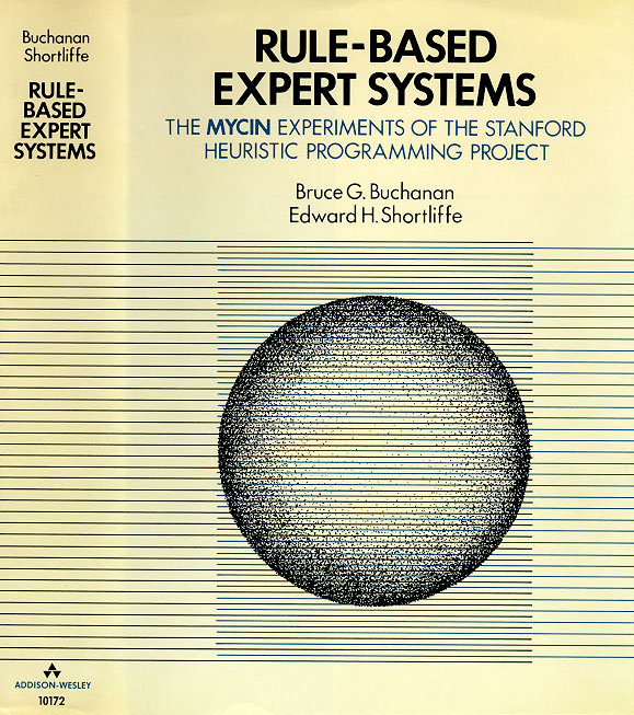
MYCIN was an early backward chaining
expert system that used artificial intelligence to identify bacteria causing severe
infections - MYCIN operated using a fairly simple inference engine and a knowledge
base of ~600 rules. - MYCIN was developed over five or six years in the early 1970s
at Stanford University. It was written in Lisp
Dendral was an artificial intelligence
project of the 1960s for the specific task of helping organic chemists in identifying
unknown organic molecules by analyzing their mass spectra and using knowledge of
chemistry. This software is considered the first expert system because it automated
the decision-making process and problem-solving behavior of organic chemists.

Although symbolic AI proved suitable to solve well-defined, logical problems, such as playing chess, it turned out to be intractable to figure out explicit rules for solving more complex, fuzzy problems, such as image classification, speech recognition, and language translation. A new approach arose to take symbolic AI’s place: Machine Learning.
Machine Learning
Machine learning arises from the question: could a computer go beyond “what we know how to order it to perform” and learn on its own how to perform a specified task? Could a computer surprise us? Rather than programmers crafting data-processing rules by hand, could a computer automatically learn these rules by looking at data?
This question opened the door to a new programming paradigm. In classical programming , the paradigm of symbolic AI, humans input rules (a program) and data to be processed according to these rules, and out come answers. With Machine Learning, humans input data as well as the answers expected from the data, and out come the rules. These rules can then be applied to new data to produce original answers.

Using data to predict something can be categorized as Machine Learning, a very simple example of this is to develop a linear regression model based, for example, on several mice weight and size measurements and use it predict the size of a new mouse based on its weight. In general, to do Machine Learning, we need three things:
- Input data points: for instance, if the task is speech recognition, these data points could be sound files of people speaking. If the task is image tagging, they could be pictures.
- Examples of the expected output: in a speech-recognition task, these could be human-generated transcripts of sound files. In an image task, expected outputs could be tags such as “dog,” “cat,” and so on.
- A way to measure whether the algorithm is doing a good job: this is necessary in order to determine the distance between the algorithm’s current output and its expected output. The measurement is used as a feedback signal to adjust the way the algorithm works. This adjustment step is what we call learning.
The central problem in Machine Learning is to meaningfully transform data, this is, to learn useful representations of the input data at hand, representations that would get us closer to the expected output. A representation is, at its core, a different way to look at data—to represent or encode data. Machine Learning models are all about finding appropriate representations for their input data transformations of the data that make it more amenable to the task at hand, such as a classification task.
Learning by changing representations
Consider a number of points distributed in a xy-coordinate system. Some of them are white and some are black.
And we are given the task to develop an algorithm to calculate the probability of the point being black or white given its x-y coordinates. In this case,
- The inputs are the coordinates of our points
- The expected outputs are the colours of our points
- The measure of success would be the percentage of points correctly classified
One way to solve the problem is by applying a coordinate change (a new representation of our data). This new representation would allow us to classify our points with a more simple set of rules: “Black points are those such that x>0”
In this case, we defined the coordinate change by hand. But if instead we tried systematically searching for different possible coordinate changes, and used as feedback the percentage of points being correctly classified, then we would be doing Machine Learning. Learning, in this context, describes an automatic search process for better representations.
Coordinate change Better representation


All Machine Learning algorithms consist of automatically finding such transformations that turn data into more useful representations for a given task. These operations can be coordinate changes, as you just saw, or linear projections, translations, nonlinear operations, and so on. Machine Learning algorithms aren’t usually creative in finding these transformations; they’re merely searching through a predefined set of operations, also called a hypothesis space.
With the previous description in mind, we can summarize Machine Learning as:
the field of study that gives computers the ability to learn without being explicitly programmed. —Arthur Samuel, 1959
Or more formally:
A computer program is said to learn from experience E with respect to some task T and some performance measure P, if its performance on T, as measured by P, improves with experience E. —Tom Mitchell, 1997
A machine-learning system is trained rather than explicitly programmed. It is presented with many examples relevant to a task, and it finds statistical structure in these examples that eventually allows the system to come up with rules for automating the task.
When to use Machine Learning
Machine Learning methods are great when:
- the solution of a problem requires lots of parameter tweaking and/or writing long lists of rules.
- there is no known optimal solution for the problem at hand.
- the problem requires adapting to constantly changing data.
- we wish to obtain more insights about complex problems and large amounts of data.
Common Machine Learning problems
There are many classes and subclasses of Machine Learning problems based on what the prediction task looks like. Some of the most common ones include:
- Classification - We want to predict one of several options. The possible outcomes are called classes. The MNIST problem is a 10 classes classification problem.
- Regression - We want to predict a continuous value. For example, mice weight given its size.
- Clustering: The goal is to split up the data in such a way that points within a single cluster are very similar and points in different clusters are different.
- Association rule learning - Helpful to infer likely association patterns in data.
- Structured output - Useful to create complex output.
- Ranking - The goal is to retrieve answers to a particular query, ordered by their relevance.
- Recommenders: Provide suggestions to users based on their preferences.
Types of Machine learning
Although there is no formal Machine Learning classification system yet, they are commonly described and classified in broad categories based on:
- How much human supervision is required. There are three major categories:
- Supervised learning: this method requires feeding the algorithm with “right” answers or solutions, also known as labels. Some of the most important supervised learning algorithms: k-Nearest Neighbours, Linear Regression, Logistic Regression, Support Vector Machines (SVMs), Decision Trees and Random Forests, Neural networks.
- Unsupervised learning: in contrast, in this algorithm the system tries to learn without a teacher, this is, with unlabelled data. Some of the most important unsupervised learning algorithms are: Clustering (K-Means, DBSCAN, Hierarchical Cluster Analysis (HCA)), Anomaly detection and novelty detection (One-class SVM, Isolation Forest), Visualization and dimensionality reduction (Principal Component Analysis (PCA), Kernel PCA, Locally-Linear Embedding (LLE), t-distributed Stochastic Neighbour Embedding (t-SNE)), Association rule learning (Apriori, Eclat).
- Semisupervised learning: these algorithms are able to work with some partially labeled training data, typically lots of unlabelled data and a few bits of labelled data. Most semisupervised learning algorithms are combinations of unsupervised and supervised algorithms.
- Reinforcement Learning
- Weather the model can learn incrementally or requires reprocessing entire datasets.
There are two major categories:
- Batch learning: This is also known as offline learning. In here the system is trained using all available data (which typically is both time and computationally expensive). Once the system is trained, it is launched in production runs where it applies what it learned but without adding any new knowledge.
- Online (incremental) learning: also known as online learning. In here the system can be trained incrementally by feeding it small data batches. This type of learning process is more useful where limited computational resources are available (e.g. when a huge database cannot be entirely contained in the machine’s memory).
- Weather the model is able to find new patterns in the data or relies on comparing
new data points to known data points.
- Instance-based learning: the system relies completely on the already learned examples and a similarity measure to generalize to new observed cases. Not the most sophisticated method, but can produce good results.
- Model-based learning: the system builds a model using a set of examples and then use it to make predictions. Depending on the model complexity there will typically be a number of parameters that need to be tuned by the system (using some kind of performance measurement) to find a set that makes the model perform best.
Main challenges
- Insufficient Quantity of Training Data: Machine Learning algorithms required high amounts of data to work properly, typically in the order of thousands of examples even for fairly simple problems and of millions for more complex problems (image or speech recognition).
- Nonrepresentative Training Data: The predictions made by a Machine Learning model depend not only on the amount of data provided to the algorithm but also on its significance. If the data is not representative of the samples the model will encounter in real life, the predictions cannot be accurate either.
- Poor-Quality Data: And related with the previous point, if the data contains a high number of errors (caused for example by noise, incomplete samples, poor measurement equipment), the algorithm will struggle to find patterns in the data.
- Irrelevant Features: In the other hand, providing more data (even high-quality data) does not guarantee a more accurate model, especially if the additional data describes unimportant aspects of the samples.
- Overfitting the Training Data: This can happen when using a relatively complex model that might be able to describe better the training data set but fails when exposed to real samples. A typical solution is to reduce the model complexity.
- Underfitting the Training Data: The opposite of creating an overfitting model is creating an underfitting one and this typically happens when the model is too simple to learn the underlying structure of the data.
Computational frameworks
Deep learning frameworks allow a user to define networks either via a config (like Caffe) or programmatically like Theano, Tensorflow, or Torch. Furthermore, the programming language exposed to define networks might vary, like Python in the case of Theano and Tensorflow or Lua in the case of Torch. An additional variation on them is whether the framework provides define-compile-execute semantics or dynamic semantics (as in the case of PyTorch).
- Sci-Kit Learn: is an open source project, meaning that it is free to use and distribute, and anyone can easily obtain the source code to see what is going on behind the scenes. The scikit-learn project is constantly being developed and improved, and it has a very active user community. It contains a number of state-of-the-art machine learning algorithms, as well as comprehensive documentation about each algorithm. scikit-learn is a very popular tool, and the most prominent Python library for machine learning. It is widely used in industry and academia, and a wealth of tutorials and code snippets are available online.
- PyTorch: is an open source machine learning library based on the Torch library, used for applications such as computer vision and natural language processing, primarily developed by Facebook’s AI Research lab (FAIR). is an optimized tensor library for deep learning using GPUs and CPUs. PyTorch is very well suited for research purposes as it makes developing and experimenting with new deep learning architectures relatively easy.
- Tensorflow: allows users to define mathematical functions via computational graphs and to compute their gradients. Tensorflow is conceptually similar to Theano, and Keras uses both of them as back ends. it has strong backing from industry leaders such as Google. At its essence, Tensorflow allows users to define mathematical functions on tensors (hence the name) using computational graphs and to compute their gradients.
- Keras: is a library that provides highly powerful and abstract building blocks to build Deep and Machine Learning systems. The building blocks Keras provides are built using Theano as well as TensorFlow. Keras supports both CPU and GPU computation and is a great tool for quickly prototyping ideas.
- CNTK: is an open-source toolkit for commercial-grade distributed deep learning. It describes neural networks as a series of computational steps via a directed graph. CNTK allows the user to easily realize and combine popular model types such as feed-forward DNNs, convolutional neural networks (CNNs) and recurrent neural networks (RNNs/LSTMs).
- Theano: is a Python library for defining mathematical functions (operating over vectors and matrices), and computing the gradients of these functions. Theano allows the user to define mathematical expressions that encode loss functions and, once these are defined, Theano allows the user to compute the gradients of these expressions.
- Caffe: a deep learning framework made with expression, speed, and modularity in mind. It is developed by Berkeley AI Research (BAIR) and by community contributors.
References
Some further reading to learn more about machine and deep learning.
- Aurélien Géron (2019) Hands-On Machine Learning with Scikit-Learn, Keras, and Tensorflow Concepts, Tools, and Techniques to Build Intelligent Systems. 2nd ed. US: O’Reilly.
- Andreas C. Müller & Sarah Guido (2016) Introduction to Machine Learning with Python A Guide for Data Scientists. 1st ed. US: O’Reilly.
- Francois Chollet (2018) Deep Learning with Python. 1st ed. New York: Manning Publications.
- Delip Rao & Brian McMahan (2019) Natural Language Processing with PyTorch Build Intelligent Language Applications Using Deep Learning. 1st ed. US: O’Reilly.
- Ian Pointer (2019) Programming PyTorch for Deep Learning. 1st ed. US: O’Reilly.
Further training
Some other sources with training material for DL and ML applications:
- TensorFlow - Learn Machine Learning
- Scikit Learn Tutorials
- Coursera - DeepLearning.AI TensorFlow Developer Professional Certificate
- Coursera - Machine Learning
- Udacity - Intro to TensorFlow for Deep Learning
- Yann LeCun’s Deep Learning Course at CDS
- MIT Courseware Linear Algebra
- CS224n: Natural Language Processing with Deep Learning
- CALTECH - Learning From Data - Machine Learning Course
- UC Berkeley - Full Stack Deep Learning
- Stanford University - Introduction to Robotics
- Linear Algebra Review
- Carnegie Melon University - Math Background for Machine Learning
Key Points
Machine Learning is the science of getting computers to learn, without being explicitly programmed.
Machine Learning main objective is to find new useful representation that help understand hidden patterns in data.
There are several ways to classify machine learning algorithms based on the problem they are trying to solve, how is data processed and how much human supervision is required.
Scikit Learn - The Iris Dataset
Overview
Teaching: 60 min
Exercises: 0 minQuestions
Use Scikit Learn to build a simple classification Machine Learning model.
Objectives
Understand the use of the k-neareast neighbours algorithm.
Familizarize with using subsets of the features available in our training set.
Plot decision boundaries in classification algorithms.
In this lesson we will use a popular machine learning example, the Iris dataset, to understand some of the most basic concepts around machine learning applications. For this, we will employ Scikit-learn one of the most popular and prominent Python library for machine learning. Scikit-learn comes with a few standard datasets, for instance the iris and digits datasets for classification and the diabetes dataset for regression, you can find more information about these and other datasets in the context of Scikit-learn usage here.
The Iris Dataset
The data set consists of 50 samples from each of three species of Iris (Iris setosa, Iris virginica and Iris versicolor). Four features were measured from each sample: the length and the width of the sepals and petals, in centimeters. You can find out more about this dataset here and here.
Features
In machine learning datasets, each entity or row here is known as a sample (or data point), while the columns—the properties that describe these entities—are called features.
To start our work we can open a new Python session and import our dataset:
from sklearn.datasets import load_iris
iris_dataset = load_iris()
Datasets
In general, in machine learning applications, a dataset is a dictionary-like object that holds all the data and some metadata about the data. In particular, when we use Scikit-learn data loaders we obtain an object of type Bunch:
type(iris_dataset)sklearn.utils.BunchThis type of object is a container that exposes its keys as attributes. You can find out more about Scikit-learn Bunch objects here.
Take a look at the keys in our newly loaded dataset:
print("Keys of iris_dataset: \n{}".format(iris_dataset.keys()))
Keys of iris_dataset:
dict_keys(['data', 'target', 'frame', 'target_names', 'DESCR', 'feature_names', 'filename'])
The dataset consists of the following sections:
- data: contains the numeric measurements of sepal length, sepal width, petal length, and petal width in a NumPy array. The array contains 4 measurements (features) for 150 different flowers (samples).
- target: contains the species of each of the flowers that were measured, also as a NumPy array. Each entry consists of a integer number in the set 0, 1 or 2.
- target_names: contains the meanings of the numbers given in the target_names array: 0 means setosa, 1 means versicolor, and 2 means virginica.
- DESCR: a short description of the dataset.
- feature_names: a list of strings, giving the description of each feature in data.
- filename: location where the dataset is stored.
And we can explore the contents of these sections:
print("First five columns of data:\n{}".format(iris_dataset['data'][:5]))
print("\n")
print("Targets:\n{}".format(iris_dataset['target'][:]))
print("\n")
print("Target names:\n{}".format(iris_dataset['target_names']))
print("\n")
print("Feature names:\n{}".format(iris_dataset['feature_names']))
print("\n")
print("Dataset location:\n{}".format(iris_dataset['filename']))
First five columns of data:
[[5.1 3.5 1.4 0.2]
 [4.9 3.  1.4 0.2]
 [4.7 3.2 1.3 0.2]
 [4.6 3.1 1.5 0.2]
 [5.  3.6 1.4 0.2]]


Targets:
[0 0 0 0 0 0 0 0 0 0 0 0 0 0 0 0 0 0 0 0 0 0 0 0 0 0 0 0 0 0 0 0 0 0 0 0 0
 0 0 0 0 0 0 0 0 0 0 0 0 0 1 1 1 1 1 1 1 1 1 1 1 1 1 1 1 1 1 1 1 1 1 1 1 1
 1 1 1 1 1 1 1 1 1 1 1 1 1 1 1 1 1 1 1 1 1 1 1 1 1 1 2 2 2 2 2 2 2 2 2 2 2
 2 2 2 2 2 2 2 2 2 2 2 2 2 2 2 2 2 2 2 2 2 2 2 2 2 2 2 2 2 2 2 2 2 2 2 2 2
 2 2]


Target names:
['setosa' 'versicolor' 'virginica']


Feature names:
['sepal length (cm)', 'sepal width (cm)', 'petal length (cm)', 'petal width (cm)']


Dataset location:
/home/vagrant/anaconda3/envs/deep-learning/lib/python3.7/site-packages/sklearn/datasets/data/iris.csv
In particular, try printing the content of the DESCR key:
print(iris_dataset['DESCR'])
.. iris_dataset:

Iris plants dataset
--------------------

**Data Set Characteristics:**

    :Number of Instances: 150 (50 in each of three classes)
    :Number of Attributes: 4 numeric, predictive attributes and the class
    :Attribute Information:
        - sepal length in cm
        - sepal width in cm
        - petal length in cm
        - petal width in cm
        - class:
                - Iris-Setosa
                - Iris-Versicolour
                - Iris-Virginica

    :Summary Statistics:

    ============== ==== ==== ======= ===== ====================
                    Min  Max   Mean    SD   Class Correlation
    ============== ==== ==== ======= ===== ====================
    sepal length:   4.3  7.9   5.84   0.83    0.7826
    sepal width:    2.0  4.4   3.05   0.43   -0.4194
    petal length:   1.0  6.9   3.76   1.76    0.9490  (high!)
    petal width:    0.1  2.5   1.20   0.76    0.9565  (high!)
    ============== ==== ==== ======= ===== ====================

    :Missing Attribute Values: None
    :Class Distribution: 33.3% for each of 3 classes.
    :Creator: R.A. Fisher
    :Donor: Michael Marshall (MARSHALL%PLU@io.arc.nasa.gov)
    :Date: July, 1988

The famous Iris database, first used by Sir R.A. Fisher. The dataset is taken
from Fisher's paper. Note that it's the same as in R, but not as in the UCI
Machine Learning Repository, which has two wrong data points.

This is perhaps the best known database to be found in the
pattern recognition literature.  Fisher's paper is a classic in the field and
is referenced frequently to this day.  (See Duda & Hart, for example.)  The
data set contains 3 classes of 50 instances each, where each class refers to a
type of iris plant.  One class is linearly separable from the other 2; the
latter are NOT linearly separable from each other.

.. topic:: References

   - Fisher, R.A. "The use of multiple measurements in taxonomic problems"
     Annual Eugenics, 7, Part II, 179-188 (1936); also in "Contributions to
     Mathematical Statistics" (John Wiley, NY, 1950).
   - Duda, R.O., & Hart, P.E. (1973) Pattern Classification and Scene Analysis.
     (Q327.D83) John Wiley & Sons.  ISBN 0-471-22361-1.  See page 218.
   - Dasarathy, B.V. (1980) "Nosing Around the Neighborhood: A New System
     Structure and Classification Rule for Recognition in Partially Exposed
     Environments".  IEEE Transactions on Pattern Analysis and Machine
     Intelligence, Vol. PAMI-2, No. 1, 67-71.
   - Gates, G.W. (1972) "The Reduced Nearest Neighbor Rule".  IEEE Transactions
     on Information Theory, May 1972, 431-433.
   - See also: 1988 MLC Proceedings, 54-64.  Cheeseman et al"s AUTOCLASS II
     conceptual clustering system finds 3 classes in the data.
   - Many, many more ...
Test vs training sets
To assess the model’s performance, we show it new data (data that it hasn’t seen before) for which we have labels. This is usually done by splitting the labeled data we have collected (here, our 150 flower measurements) into two parts. One part of the data is used to build our machine learning model, and is called the training data or training set. The rest of the data will be used to assess how well the model works; this is called the test data, test set, or hold-out set.
Unfortunately, we cannot use the data we used to build the model to evaluate it. This is because our model could always simply remember the whole training set (overfitting), and will therefore always predict the correct label for any point in the training set. This “remembering” does not indicate to us whether our model will generalize well (in other words, whether it will also perform well on new data).
Training
Scikit-learn’s train_test_split function allow us to shuffle and split the dataset in a single line. The function takes a sequence of arrays (the arrays must be of the same length) and options to specify how to split the arrays. By default, the function extracts 75% of the rows in the arrays as the training set while the remaining 25% of rows is declared as the test set. Deciding how much data you want to put into the training and the test set respectively is somewhat arbitrary, but using a test set containing 25% of the data is a good rule of thumb. The function also allow us to control the shuffling applied to the data before applying the split with the option random_state, this ensures reproducible results.
from sklearn.model_selection import train_test_split

X_train, X_test, y_train, y_test = train_test_split(
        iris_dataset['data'], iris_dataset['target'], test_size=0.25, random_state=0)
print("X_train shape: {}".format(X_train.shape))
print("y_train shape: {}".format(y_train.shape))
print("X_test shape: {}".format(X_test.shape))
print("y_test shape: {}".format(y_test.shape))
X_train shape: (112, 4)
y_train shape: (112,)
X_test shape: (38, 4)
y_test shape: (38,)
We can use Pandas’ plotting function scatter_matrix that draws a matrix of scatter plots to visualize our data. This function takes a dataframe and plots each variable contained within, against each other. The first step is import Pandas and transfor our Numpy array into a Pandas dataframe:
import pandas as pd
iris_dataframe = pd.DataFrame(X_train, columns=iris_dataset.feature_names)
grr = pd.plotting.scatter_matrix(iris_dataframe, c=y_train, figsize=(15, 15), marker='o',hist_kwds={'bins': 20}, s=60, alpha=.8)
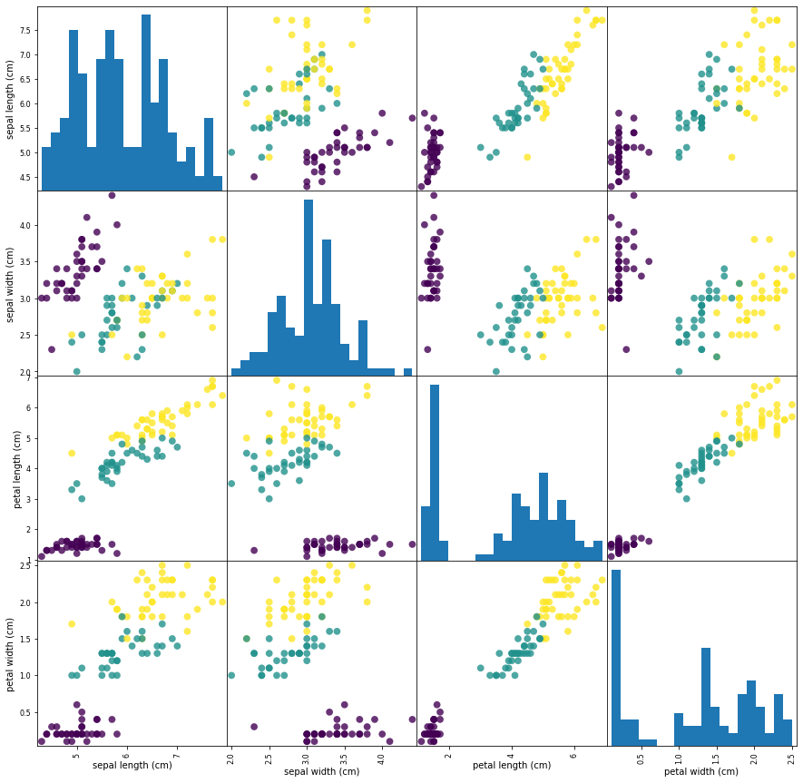
The diagonal in the image shows the distribution of the three numeric variables of our example data. In the other cells of the plot matrix, we have the scatter plots of each variable combination of our dataframe. Take a look at Pandas’ scatter_matrix documentation to find out more about the options we have used. Keep in mind as well that Pandas’ scatter_matrix makes use of Matplotlib’s scatter function under the hood to perform the actual plotting and that we have passed a couple of arguments to this function in our previous command, specifically point color and size options. Find out more at Matplotlib’s scatter function documentation.
Back to the plots, we can see that the three classes seem to be relatively well separated using the sepal and petal measurements. This means that a machine learning model will likely be able to learn to separate them.
Building the model
There are many classification algorithms in scikit-learn that we could use. Here we will use a k-nearest neighbors classifier, which is easy to understand. Neighbors-based classification algorithms are a type of instance-based learning that does not attempt to construct a general internal model, but simply stores instances of the training data. Classification is computed from a simple majority vote of the nearest neighbors of each point: a query point is assigned the data class which has the most representatives within the nearest neighbors of the point.
Building this model only consists of storing the training set. To make a prediction for a new data point, the algorithm finds the point in the training set that is closest to the new point. Then it assigns the label of this training point to the new data point.
from sklearn.neighbors import KNeighborsClassifier
n_neighbors=1
knn = KNeighborsClassifier(n_neighbors=1)
knn becomes an object that contains the algorithm used to build the model using the training dataset as well as to make predictions from new data points. Now we can train our model using the training dataset. We could use all the features of training data set our just a sub set. In this case, to facilitate later visualization, we will only use two features: petal length (cm) and petal width (cm):
knn.fit(X_train[:,2:], y_train)
Plot the decision boundaries
Once again, in order to understand how the model classifies new points, it could be useful to visualize it. For this we can use matplotlib library and plot our training data set on top of a coloured domain in which each color represents a category in our model.
import numpy as np
from matplotlib.colors import ListedColormap
import matplotlib.pyplot as plt

x_min,x_max = X_train[:,2].min() - 1, X_train[:,2].max()+ 1
y_min,y_max = X_train[:,3].min() - 1, X_train[:,3].max()+ 1
h=0.02
xx,yy = np.meshgrid(np.arange(x_min,x_max,h),np.arange(y_min,y_max,h))
Z = knn.predict(np.c_[xx.ravel(), yy.ravel()])
Z = Z.reshape(xx.shape)

cmap_bold = ListedColormap(['darkorange', 'c', 'darkblue'])
cmap_light=ListedColormap(['orange', 'cyan', 'cornflowerblue'])

fig = plt.figure()
ax1 = fig.add_subplot(111)
ax1.pcolormesh(xx, yy, Z, cmap=cmap_light, shading='gouraud')
for target in iris_dataset.target_names:
    index=np.where(iris_dataset.target_names==target)[0][0]
    ax1.scatter(X_train[:,2][y_train==index],X_train[:,3][y_train==index],
                cmap=cmap_bold,edgecolor='k', s=20, label=target)
ax1.set_xlim(x_min,x_max)
ax1.set_ylim(y_min,y_max)
ax1.legend()
ax1.set_xlabel("petal length (cm)")
ax1.set_ylabel("petal width (cm)")
ax1.set_title("3-Class classification (k = %i, weights = '%s')"
              % (n_neighbors, 'uniform'))
plt.show()
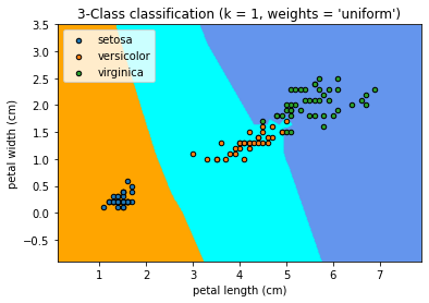
This figure show us the regions where new data points would be classified based on their petal length and width measurements.
Making predictions
With out newly build model, we can now make predictions on new data for which we would like to find the correct labels. Assume you found an iris in the park with a sepal length of 4 cm, a sepal width of 3.5 cm, a petal length of 1.2 cm, and a petal width of 0.5 cm.
new_data=np.array([[4,3.5,1.2,0.5]])
prediction = knn.predict(new_data[:,2:])
print("Prediction: {}".format(prediction))
print("Predicted target name: {}".format(iris_dataset['target_names'][prediction]))
Validate the model
Our model predicts that the iris found in the park belongs to the setosa species. How sure can we be that this is the correct answer? For this, we need to validate our model using the data we set apart for this purpose in which we know the right species for each flower in the set (remember we are working only with 2 features from our data set).
y_pred = knn.predict(X_test[:,2:])
print("Test set predictions:\n {}".format(y_pred))
The above command give us the following output that represents the class for each entry in the validation dataset:
Test set predictions:
 [2 1 0 2 0 2 0 1 1 1 2 1 1 1 1 0 1 1 0 0 2 1 0 0 2 0 0 1 1 0 2 1 0 2 2 1 0 2]
And now we can compare the above predicted classes with their actual values and obtain a measure (accuracy) of how well our model works.
print("Test set score: {:.2f}".format(knn.score(X_test[:,2:], y_test)))
Test set score: 0.97
Now we could say that we are 97% sure that the iris we found at the park belongs to the setosa species. You can try to use a different set of features or maybe all of them and see if you can improve this value (be aware of overfitting your model).
Key Points
k-Nearest Neighbors is a simple classification algorithm in which predictions a new data point to the closest data points in the training dataset.
It is not necessary to use all the features in our training dataset. We can use different combinations to try to achive better results.
Scikit Learn - Linear Model
Overview
Teaching: 45 min
Exercises: 0 minQuestions
Use Scikit Learn to build a simple linear regression machine learning problem.
Objectives
Familiarize with the basic steps involved in building a machine learning model.
Test our machine learning tools and environment.
GDP and happiness
We will start building a very simple model to predict people Happiness (as measured by the OECD) based on the country’s GDP (as provided by the IMF). This is also called model-based learning. For this course we will use Scikit-Learn but other libraries should provide similar functionalities.
Obtaining and working with data
When developing Machine Learning applications you will likely need to work with databases either by creating them yourself or obtaining some already available. Depending on the field and stage of your research, the databases can range from a few megabytes to several hundreds gigabytes and ever bigger. At that point you’ll likely need to consider carefully (even more if the database has data protection requirements) how best to manage storage requirements in order to optimize available resources in your work system. Do not hesitate to contact your system administrators to discuss further any doubts or concerns that you might have.
Luckily for this training the databases we will be working with are publicly available from the OECD’s Better Life Index) and the IMF’s GDP per capita) and only occupy a few megabytes. You can also find them in the zip file provided for this training course.
Start by loading some python libraries.
import matplotlib.pyplot as plt
import numpy as np
import pandas as pd
import sklearn.linear_model
Continue by loading the data as Pandas dataframes. For this you need to provide the corresponding file locations, for example:
file_gdp="gdp-bli/gdp_per_capita_2014-2025.csv"
file_happy="gdp-bli/BLI_25112020150937807.csv"

df_gdp=pd.read_csv(file_gdp,thousands=',',delimiter='\t',encoding='latin1',na_values='n/a')
df_happy=pd.read_csv(file_happy,thousands=',')
You can take a look at the data we just loaded with the head dataframe function, for example, to print the first 5 rows in the GDP dataframe:
rows=5
df_gdp.head(rows)
Preparing our data
Next we define a few helper functions to extract subsets of our dataset.
OECD Better Life Index dataset
The following function extracts data based on an indicator and an inequality group and then returns a dataframe with the indicator data per country:
def oecd_bli_indicator(data,indicator):
    """
    Process OECD Better Life Index data
    Extract a specific "Indicator" from the dataset
    Each indicator in the dataset is aggregated to take into
    account the inequalities of different population groups:

    "MN"  - Men
    "WMN" - Women
    "HGH" - High socio-economic status
    "LW"  - Low socio-economic status
    "TOT" - All population

    We use TOT in this example, but feel free to check the
    results with different groups.
    """
    assert indicator in data["Indicator"].unique(), "{} is not available in dataset".format(indicator)

    result = data[(data["INEQUALITY"]=="TOT") & (data["Indicator"]==indicator)][["Country","Value"]]
    result = result.rename(columns={"Value":indicator})
    result = result.set_index("Country").sort_values(by=["Country"])

    return result
In this example we use Life satisfaction as indicator and Total as inequality group, but feel free to try other parameters.
indicator = "Life satisfaction"
inequality = "MN"
bli_data = oecd_bli_indicator(df_happy,indicator,inequality)
Gross Domestic Product dataset from the International Monetary Fund
The function below simply selects a column from the dataset corresponding to a year and returns a dataframe with GDP information per country for that year.
def gdp_extract_year(data,year):
    """
    Process Gross Domestic Product data from IMF
    Extract data column corresponding to a specific year
    rename column and set a new index
    """
    assert year in data.columns, "{} is not available in dataset".format(year)
    gdp_year = data[["Country",year]]
    gdp_year = gdp_year.rename(columns={year:"GDP per capita {}".format(year)})
    gdp_year = gdp_year.set_index("Country")
    return gdp_year
In this example we work with year 2020, but try with other years and check if you obtain similar results.
year = "2020"
gdp_data = gdp_extract_year(df_gdp,year)
Merging our datasets
With our datasets ready, the next step is merging them based on country name. The function below is in charge of this:
def merge_by_country(gdp_data,bli_data):
    """
    Merge both datasets by country.
    We only keep those countries common to both datasets
    """
    merged_data = pd.merge(left=bli_data, right=gdp_data,left_index=True, right_index=True)
    return merged_data
Note that not all countries appear in both datasets and we only keep information for countries common to both datasets. This produces our final input dataset.
input_data = merge_by_country(gdp_data,bli_data)
Split training and testing datasets
To divide our input data in two sets for training and testing we can use Scikit Learn function train_test_split as in the previous lesson.
x_training, x_testing, y_training, y_testing = train_test_split(input_data["GDP per capita {}".format(year)].to_numpy(),
                                                                input_data["Life satisfaction"].to_numpy(),
                                                                test_size=0.25, random_state=0)
Visualising our data
Before building our model, it can be useful to visualise the data to gain insights about what type of models could be better suited for it. For this we can use the helper function below, which is prepared to plot both training and testing datasets, and a regression line using a slope (m) and intercept (b) coefficients, if provided.
import matplotlib.pyplot as plt
def scatter_plot(x_train,y_train,x_test=None,y_test=None,m=None,b=None):
    #plot training data
    plt.scatter(x_train,y_train,color='red')

    # plot testing data if given
    if (x_test is not None) and (y_test is not None):
        plt.scatter(x_test,y_test,color='green')

    # plot model's predicted line if coefficients given
    if (m is not None) and (b is not None):
        x = np.arange(0,100000)
        plt.plot(x, b + m * x, '-')

    plt.xlabel("GDP per capita (2020)")
    plt.ylabel("Life satisfaction")
    plt.xlim([0,100000])
    plt.ylim([0,10])
We can test our function by plotting the training dataset:
scatter_plot(x_training,y_training)
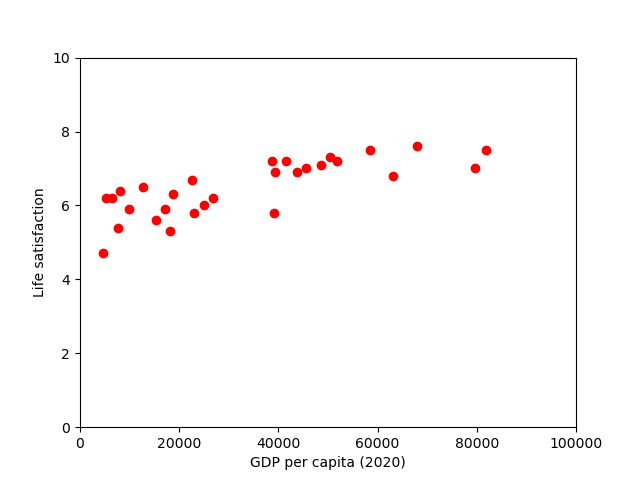
There does seem to be a trend here! Although the data is noisy (i.e., partly random), it looks like life satisfaction goes up more or less linearly as the country’s GDP per capita increases. So we decide to model life satisfaction as a linear function of GDP per capita.
Building the model
Based on the above observations, we select a linear model of life satisfaction with just one attribute, GDP per capita:
model = sklearn.linear_model.LinearRegression()
With the model selected, the next step is to fit it to the data. The calculations performed in this step are model dependent, for example, for a linear model it involves calculating a set of coefficients to minimize the residual sum of squares between the observed targets in the dataset, and the targets predicted by the linear approximation.
model.fit(np.c_[x_training], np.c_[y_training])
And we can access the estimated value for the model key parameters (which parameters are available also depends on the selected model).
print(f"model's intercept: {model.intercept_[0]}")
print(f"model's slope    : {model.coef_[0][0]}")
model's intercept: 5.77342747430831
model's slope    : 2.025726170863078e-05
It might be useful to plot our model alongside our data, including the trend line:
scatter_plot(x_training,y_training,
            m=model.coef_[0][0],b=model.intercept_[0])
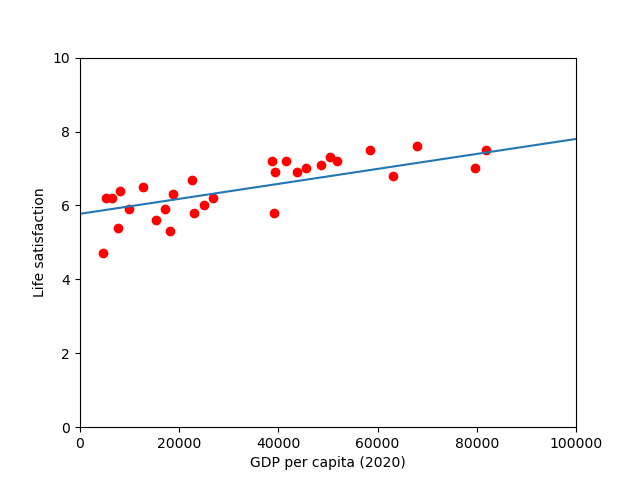
there seems to be a good fit between the training data and the trend line predicted by the model, however, we still need to compare with out test dataset.
Validating and making predictions
After we have trained our model, we should perform some validation checks using the labelled data we saved for this purpose:
model.score(np.c_[x_testing],np.c_[y_testing])
0.5010135842893668
Always helpful to have some visual aids to compare how well our model does against the validation data
scatter_plot(x_training,y_training,
             x_testing,y_testing,
             model.coef_[0][0],model.intercept_[0])
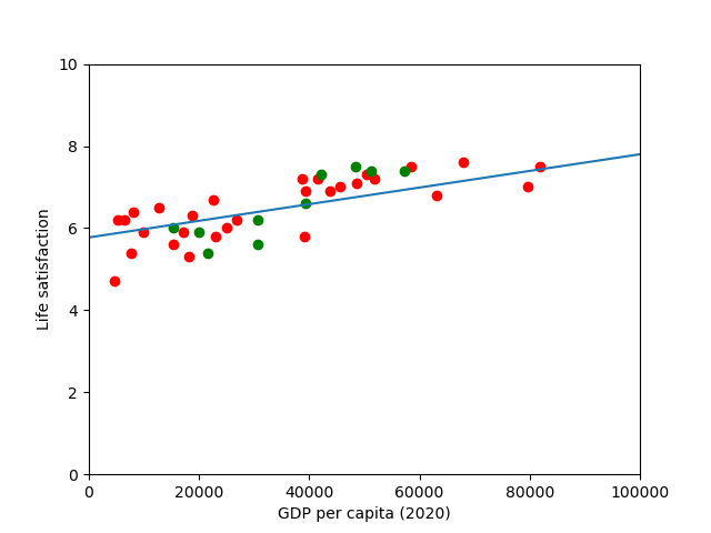
Visually, it appears as like our model is reasonably good at predicting values in our test dataset, however, a coefficient of determination of 0.50 might not be great depending on the field. At this point it might be worth thinking about using alternative indicators (employment rate, health, air) or additional features to improve our model if needed.
Key Points
Python is a very useful programming language to develop machine learning applications
Scikit Learn together with Numpy, Pandas and Matplotlib form a popular machine learning environment.
Linear regression is one of the most simple and useful machine learning algorithms in which the model makes a prediction by simply computing a weighted sum of the input features, plus a constant called the intercept term.
Keras & Tensorflow - The MNIST dataset
Overview
Teaching: 30 min
Exercises: 0 minQuestions
Building a first Deep Learning model to recognize handwritten digits.
Objectives
FIX
Deep Learning is a subset of Machine Learning that is inspired by the brain’s architecture to build an intelligent machine through the use of artificial neural networks (ANNs) which are the very core of Deep Learning. They are versatile, powerful, and scalable, making them ideal to tackle large and highly complex Machine Learning tasks, such as classifying billions of images and running speech recognition services.
As other Machine Learning algorithms, ANNs have their own set of parameters that need to be specified and tweak in order to create, train and use a model. We will try to exemplify these parameters and steps through solving a very simple deep learning problem. For this we will use Keras API which is a beautifully designed and simple high-level API for building, training, evaluating and running neural networks. Despite its simplicity it is flexible enough to allow you to build a wide variety of neural network architectures.
The MNIST dataset.
We will use the MNIST dataset, a classic machine learning algorithm. The dataset consists of 60,000 training images and 10,000 testing images. Each element in the dataset correspond to a grayscale image of handwritten digits (28x28 pixels). You can think of solving MNIST, this is, classifying each number into one of 10 categories or class, as the “Hello World” of deep learning and can be used to verify that algorithms work correctly.
We can use Keras to work with MNIST since it comes preloaded as a set of four Numpy arrays:
from keras.datasets import mnist
(train_images, train_labels),(test_images, test_labels) = mnist.load_data()
If this is the first time importing mnist, Keras with try to download it from the internet.
Using TensorFlow backend.
Downloading data from https://s3.amazonaws.com/img-datasets/mnist.npz
11493376/11490434 [==============================] - 7s 1us/step
Downloading data in HPC systems
When working on HPC systems is not uncommon that compute or work nodes are close to the outside world for security reasons. In those cases, it is better to try to download any required data locally in the login or head nodes and then instruct your code how to access it.
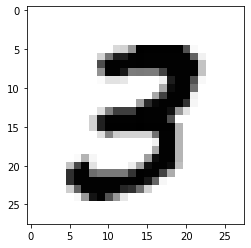
The model will learn from the training set composed by train_images and train_labels and then will be tested on the test set test_images and test_labels. The images are encoded as Numpy arrays, and the labels are an array of digits, ranging from 0 to 9. We can check which digit is placed in position 8 in the training set (remember that numpy arrays are zero-based indexed) with:
print("Digit at position 8:",train_labels[7])
3
If we wanted to see the corresponding image we could use Python’s Matplotlib:
import matplotlib.pyplot as plt
plt.imshow(train_images[7],cmap=plt.cm.binary)
We can further confirm the size of our sets:
print("Number of train images: ", train_images.shape)
print("Number of train labels: ", train_labels.shape)
print("Number of test images: ", test_images.shape)
print("Number of test labels: ", test_labels.shape)
Number of train images:  (60000, 28, 28)
Number of train labels:  (60000,)
Number of test images:  (10000, 28, 28)
Number of test labels:  (10000,)
Building the model
In deep learning algorithms we rely on ANNs which building blocks are the layer, a data processing module that works as a filter for data. Layers are in charge of extracting representations out of the data fed into them. The deep in deep learning comes from chaining together simple layers on top of each other in a kind of data distillation process.
In Keras, Models groups layers into an object with training and inference features. There are three ways to create Keras models: the sequential model, which is simply a list of layers and is limited to single input and single output layers; the functional API, which supports arbitrary model architecture and is applicable to most use cases; and a model subclassing that allows the user to everything from scratch for maximum flexibility. For this course we will use a simple sequential model. We start by importing the necessary libraries and instantiating a model.
from tensorflow.keras import models

network = models.Sequential()
A deep learning model consist of a series of stacked layers. A layer consists of a tensor-in tensor-out computation function. For this example we use two densely connected NN layers. The first one receives a layer of 28 by 28 input elements that corresponds to our images. activation is an element-wise activation function, kernel and bias are a weights matrix and a bias vector created by the layer. The first argument passed to the dense layer indicates the number of nodes in the layer, (or dimensionality of the layer’s output space).
from tensorflow.keras import layers

network.add(layers.Dense(512,activation='relu',input_shape=(28 * 28,)))
network.add(layers.Dense(10,activation='softmax'))
Dense layers implements the operation:
output = activation(dot(input, kernel) + bias)
As mentioned above, activation is a element wise function, there are several types but for this example we use two of the most common ones: relu function, that applies the rectified linear unit activation function; and the softmax function, that converts a real vector to a vector of categorical probabilities. The latter is often used as the activation for the last layer of a classification network because the result could be interpreted as a probability distribution. In this case each score will be the probability that the current digit image belongs to one out of 10 digit classes.
We can find out more details about our network with:
network.summary()
Model: "sequential_3"
_________________________________________________________________
Layer (type)                 Output Shape              Param #
=================================================================
dense_6 (Dense)              (None, 512)               401920
_________________________________________________________________
dense_7 (Dense)              (None, 10)                5130
=================================================================
Total params: 407,050
Trainable params: 407,050
Non-trainable params: 0
_________________________________________________________________
_.
Where a trainable parameter is a parameter that is learned by a network during training. These commonly are the weights and biases of the network but can refer to any other parameter that is learned during training. We can find out how many trainable parameters are in our network by counting the number of parameters within each layer and then sum them up to get the total in the network. For this we need the number of inputs to the layer, its number of outputs (equal to the number of nodes in the layer) and whether or not the layer contains biases (also equal to the number of nodes in the layer). Then we simply multiply the number of inputs and outputs and add the number biases and then add the results for all layers. These parameters are where knowledge of the network persists. If you are curious, you can take a look with:
network.get_weights()
Training
Before actually training our model, there are three parameters that need to be defined as part of a compilation step:
- Loss function: is the function that the network is required to minimize (cost or error function) or maximize (objective function).
- Optimizer: defines how the network should change its weights or learning rates to reduce the losses.
- Metrics: A list of metrics to be evaluated by the model during training and testing. ‘accuracy’ is a typically used metric in Keras models.
network.compile(optimizer='rmsprop',
                loss='categorical_crossentropy',
                metrics=['accuracy'])
The next step is to prepare our data to be fed to the model. As we are expecting the model to output the probability (between 0 and 1) that a digit belongs to 1 of 10 classes, we need to transform our data accordingly.
train_images = train_images.reshape((60000,28 * 28))
train_images = train_images.astype('float32')/255
test_images = test_images.reshape((10000,28 * 28))
test_images = test_images.astype('float32')/255
And we convert the label vectors to binary matrices for use with the categorical crossentropy loss function:
from tensorflow.keras.utils import to_categorical
train_labels = to_categorical(train_labels)
test_labels = to_categorical(test_labels)
We are finally ready to train our model by calling its fit method:
network.fit(train_images,train_labels,epochs=5,batch_size=128)
Epoch 1/5
469/469 [==============================] - 8s 16ms/step - loss: 0.2574 - accuracy: 0.9251
Epoch 2/5
469/469 [==============================] - 4s 9ms/step - loss: 0.1032 - accuracy: 0.9699
Epoch 3/5
469/469 [==============================] - 4s 9ms/step - loss: 0.0678 - accuracy: 0.9797
Epoch 4/5
469/469 [==============================] - 4s 9ms/step - loss: 0.0490 - accuracy: 0.9852
Epoch 5/5
469/469 [==============================] - 4s 9ms/step - loss: 0.0367 - accuracy: 0.9890
Notice that the model’s accuracy increases while the loss value decreases at the end of each epoch. This is the expected behaviour when training a deep learning model. The rate at which learning will occur depends on many parameters and you should try to test alternative algorithms and parameters.
Batches and Epochs
Deep learning models very often don’t process an entire dataset at once (especially when the amount of data is very large), but instead break the data into subsets called batches. For example, one batch of 256 images would simply be:
batch = train_images[:256]An entire iteration over all the training data is known as an epoch.
Validation
As we did with in our previous machine learning models, it is very useful to measure the degree of confidence we should have in our model by comparing its predictions on data for which we know the real values. For this we use our test dataset:
test_loss, test_acc = network.evaluate(test_images,test_labels)
print('test_acc:',test_acc)
313/313 [==============================] - 1s 3ms/step - loss: 0.0654 - accuracy: 0.9801
test_acc: 0.9800999760627747
Our model reached an accuracy of 0.98% for the validation data set which is slightly lower than the accuracy obtained with the training data, which is an example of overfitting.
Hopefully solving this very simple deep learning exercise will allow your quest to tackle more complex problems in your work.
Key Points
FIX
Pretrained models & Transfer Learning
Overview
Teaching: 30 min
Exercises: 0 minQuestions
FIX
Objectives
Use Keras to load a very well-trained pretrained model
Preprocess your own images to work with the pretrained model
Use the pretrained model to perform accurate inference on your own images
Prepare a pretrained model for transfer learning
Perform transfer learning with your own small dataset on a pretrained model
Further fine tune the model for even better performance
This section is taken from NVIDIA’s Deep Learning Institute workshop: “Getting started with Deep Learning”. You can find the complete course and many others at https://www.nvidia.com/en-gb/training/online/. Please note that you may need to pay for some of these courses but ask your local DLI ambassador for a promo code to get access for free.
Pre-Trained Models
Though it is often necessary to have a large, well annotated dataset to solve a deep learning challenge, there are many freely available pre-trained models that we can use right out of the box. As you decide to take on your own deep learning project, it is a great idea to start by looking for existing models online that can help you achieve your goal. A great place to explore available models is NGC. There are also many models hosted on GitHub that you can find through searching on Google.
Objectives
- Use Keras to load a very well-trained pretrained model
- Preprocess your own images to work with the pretrained model
- Use the pretrained model to perform accurate inference on your own images
An Automated Doggy Door
In this section, we will be creating a doggy door that only lets dogs (and not other animals) in and out. We can keep our cats inside, and other animals outside where they belong. Using the techniques covered so far, we would need a very large dataset with pictures of many dogs, as well as other animals. Luckily, there is a readily available model that has been trained on a massive dataset, including lots of animals.
The ImageNet challenge has produced many state-of-the-art models that can be used for image classification. They are trained on millions of images, and can accurately classify images into 1000 different categories. Many of those categories are animals, including breeds of dogs and cats. This is a perfect model for our doggy door.
Loading the Model
We will start by downloading the model. Trained ImageNet models are available to download directly within the Keras library. You can see the available models and their details here. Any of these models would work for our exercise. We will pick a commonly used one called VGG16:
from tensorflow.keras.applications import VGG16

# load the VGG16 network *pre-trained* on the ImageNet dataset
model = VGG16(weights="imagenet")
Now that it is loaded, let us take a look at the model. It looks a lot like our convolutional model from the sign language exercise. Pay attention to the first layer (the input layer) and the last layer (the output layer). As with our earlier exercises, we need to make sure our images match the input dimensions that the model expects. It is also valuable to understand what the model will return from the final output layer.
model.summary()
Model: "vgg16"
_________________________________________________________________
 Layer (type)                Output Shape              Param #
=================================================================
 input_1 (InputLayer)        [(None, 224, 224, 3)]     0

 block1_conv1 (Conv2D)       (None, 224, 224, 64)      1792

 block1_conv2 (Conv2D)       (None, 224, 224, 64)      36928

 block1_pool (MaxPooling2D)  (None, 112, 112, 64)      0

 block2_conv1 (Conv2D)       (None, 112, 112, 128)     73856

 block2_conv2 (Conv2D)       (None, 112, 112, 128)     147584

 block2_pool (MaxPooling2D)  (None, 56, 56, 128)       0

 block3_conv1 (Conv2D)       (None, 56, 56, 256)       295168

 block3_conv2 (Conv2D)       (None, 56, 56, 256)       590080

 block3_conv3 (Conv2D)       (None, 56, 56, 256)       590080

 block3_pool (MaxPooling2D)  (None, 28, 28, 256)       0

 block4_conv1 (Conv2D)       (None, 28, 28, 512)       1180160

 block4_conv2 (Conv2D)       (None, 28, 28, 512)       2359808

 block4_conv3 (Conv2D)       (None, 28, 28, 512)       2359808

 block4_pool (MaxPooling2D)  (None, 14, 14, 512)       0

 block5_conv1 (Conv2D)       (None, 14, 14, 512)       2359808

 block5_conv2 (Conv2D)       (None, 14, 14, 512)       2359808

 block5_conv3 (Conv2D)       (None, 14, 14, 512)       2359808

 block5_pool (MaxPooling2D)  (None, 7, 7, 512)         0

 flatten (Flatten)           (None, 25088)             0

 fc1 (Dense)                 (None, 4096)              102764544

 fc2 (Dense)                 (None, 4096)              16781312

 predictions (Dense)         (None, 1000)              4097000

=================================================================
Total params: 138,357,544
Trainable params: 138,357,544
Non-trainable params: 0
_________________________________________________________________
Input dimensions
We can see that the model is expecting images in the shape of (224, 224, 3) corresponding to 224 pixels high, 224 pixels wide, and 3 color channels. As we learned in our last exercise, Keras models can accept more than one image at a time for prediction. If we pass in just one image, the shape will be (1, 224, 224, 3). We will need to make sure that when passing images into our model for prediction, they match these dimensions.
Output dimensions
We can also see that the model will return a prediction of shape 1000. Remember that in our first exercise the output shape of our model was 10, corresponding to the 10 different digits. In our second exercise we had a shape of 24, corresponding to the 24 letters of the sign language alphabet that could be captured in a still image. Here, we have 1000 possible categories that the image will be placed in. Though the full ImageNet dataset has over 20,000 categories, the competition and result in pre-trained models just use a subset of 1000 of these categories. We can take a look at all of these possible categories here.
Many of the categories are animals, including many types of dogs and cats. The dogs are categories 151 through 268. The cats are categories 281 through 285. We will be able to use these categories to tell our doggy door what type of animal is at our door, and whether we should let them in or not.
Loading an Image
We will start by loading in an image and displaying it, as we have done in previous exercises.
import matplotlib.pyplot as plt
import matplotlib.image as mpimg

def show_image(image_path):
    image = mpimg.imread(image_path)
    print(image.shape)
    plt.imshow(image)
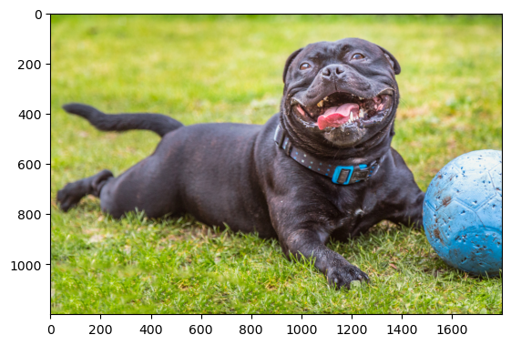
show_image("data/doggy_door_images/happy_dog.jpg")
(1200, 1800, 3)
Preprocessing the Image
Next, we need to preprocess the image so that it is ready to be sent into the model. This is just like what we did in our last exercise when we predicted on the sign language images. Remember that in this case, the final shape of the image needs to be (1, 224, 224, 3).
When loading models directly with Keras, we can also take advantage of preprocess_input methods. These methods, associated with a specific model, allow users to preprocess their own images to match the qualities of the images that the model was originally trained on. We had to do this manually yourself when performing inference with new ASL images:
from tensorflow.keras.preprocessing import image as image_utils
from tensorflow.keras.applications.vgg16 import preprocess_input

def load_and_process_image(image_path):
    # Print image's original shape, for reference
    print('Original image shape: ', mpimg.imread(image_path).shape)

    # Load in the image with a target size of 224, 224
    image = image_utils.load_img(image_path, target_size=(224, 224))
    # Convert the image from a PIL format to a numpy array
    image = image_utils.img_to_array(image)
    # Add a dimension for number of images, in our case 1
    image = image.reshape(1,224,224,3)
    # Preprocess image to align with original ImageNet dataset
    image = preprocess_input(image)
    # Print image's shape after processing
    print('Processed image shape: ', image.shape)
    return image
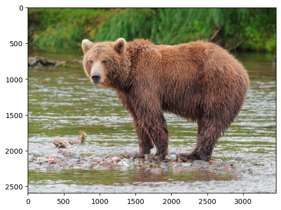
processed_image = load_and_process_image("data/doggy_door_images/brown_bear.jpg")
Original image shape:  (2592, 3456, 3)
Processed image shape:  (1, 224, 224, 3)
Make a Prediction
Now that we have our image in the right format, we can pass it into our model and get a prediction. We are expecting an output of an array of 1000 elements, which is going to be difficult to read. Fortunately, models loaded directly with Keras have yet another helpful method that will translate that prediction array into a more readable form.
from tensorflow.keras.applications.vgg16 import decode_predictions

def readable_prediction(image_path):
    # Show image
    show_image(image_path)
    # Load and pre-process image
    image = load_and_process_image(image_path)
    # Make predictions
    predictions = model.predict(image)
    # Print predictions in readable form
    print('Predicted:', decode_predictions(predictions, top=3))
Try it out on a few animals to see the results! Also feel free to upload your own images and categorize them just to see how well it works.
readable_prediction("data/doggy_door_images/happy_dog.jpg")
(1200, 1800, 3)
Original image shape:  (1200, 1800, 3)
Processed image shape:  (1, 224, 224, 3)
1/1 [==============================] - 0s 129ms/step
Downloading data from https://storage.googleapis.com/download.tensorflow.org/data/imagenet_class_index.json
35363/35363 [==============================] - 0s 1us/step
Predicted: [[('n02093256', 'Staffordshire_bullterrier', 0.4509814), ('n02110958', 'pug', 0.32263216), ('n02099712', 'Labrador_retriever', 0.09343193)]]

readable_prediction("data/doggy_door_images/brown_bear.jpg")
(2592, 3456, 3)
Original image shape:  (2592, 3456, 3)
Processed image shape:  (1, 224, 224, 3)
1/1 [==============================] - 0s 111ms/step
Predicted: [[('n02132136', 'brown_bear', 0.98538613), ('n02133161', 'American_black_bear', 0.01387624), ('n02410509', 'bison', 0.000266038)]]

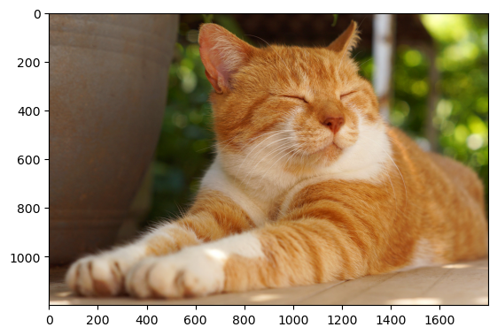
readable_prediction("data/doggy_door_images/sleepy_cat.jpg")
(1200, 1800, 3)
Original image shape:  (1200, 1800, 3)
Processed image shape:  (1, 224, 224, 3)
1/1 [==============================] - 0s 122ms/step
Predicted: [[('n02123159', 'tiger_cat', 0.7365469), ('n02124075', 'Egyptian_cat', 0.17492704), ('n02123045', 'tabby', 0.04588393)]]

Only Dogs
Now that we are making predictions with our model, we can use our categories to only let dogs in and out and keep cats inside. Remember that dogs are categories 151 through 268 and cats are categories 281 through 285. The np.argmax function can find which element of the prediction array is the top category.
import numpy as np

def doggy_door(image_path):
    show_image(image_path)
    image = load_and_process_image(image_path)
    preds = model.predict(image)
    if 151 <= np.argmax(preds) <= 268:
        print("Doggy come on in!")
    elif 281 <= np.argmax(preds) <= 285:
        print("Kitty stay inside!")
    else:
        print("You're not a dog! Stay outside!")
doggy_door("data/doggy_door_images/brown_bear.jpg")
(2592, 3456, 3)
Original image shape:  (2592, 3456, 3)
Processed image shape:  (1, 224, 224, 3)


2023-10-16 12:28:22.055577: W tensorflow/tsl/platform/profile_utils/cpu_utils.cc:128] Failed to get CPU frequency: 0 Hz


1/1 [==============================] - 0s 250ms/step
You're not a dog! Stay outside!
doggy_door("data/doggy_door_images/happy_dog.jpg")
(1200, 1800, 3)
Original image shape:  (1200, 1800, 3)
Processed image shape:  (1, 224, 224, 3)
1/1 [==============================] - 0s 117ms/step
Doggy come on in!

doggy_door("data/doggy_door_images/sleepy_cat.jpg")
(1200, 1800, 3)
Original image shape:  (1200, 1800, 3)
Processed image shape:  (1, 224, 224, 3)
1/1 [==============================] - 0s 113ms/step
Kitty stay inside!
Summary
Great work! Using a powerful pre-trained model, we have created a functional doggy door in just a few lines of code. We hope you are excited to realize that you can take advantage of deep learning without a lot of up-front work. The best part is, as the deep learning community moves forward, more models will become available for you to use on your own projects.
Clear the Memory
Before moving on, please execute the following cell to clear up the GPU memory.
import IPython
app = IPython.Application.instance()
app.kernel.do_shutdown(True)
Next
Using pretrained models is incredibly powerful, but sometimes they are not a perfect fit for your data. In the next section you will learn about another powerful technique, transfer learning, which allows you to tailer pretrained models to make good predictions for your data.
Transfer Learning
So far, we have trained accurate models on large datasets, and also downloaded a pre-trained model that we used with no training necessary. But what if we cannot find a pre-trained model that does exactly what you need, and what if we do not have a sufficiently large dataset to train a model from scratch? In this case, there is a very helpful technique we can use called transfer learning.
With transfer learning, we take a pre-trained model and retrain it on a task that has some overlap with the original training task. A good analogy for this is an artist who is skilled in one medium, such as painting, who wants to learn to practice in another medium, such as charcoal drawing. We can imagine that the skills they learned while painting would be very valuable in learning how to draw with charcoal.
As an example in deep learning, say we have a pre-trained model that is very good at recognizing different types of cars, and we want to train a model to recognize types of motorcycles. A lot of the learnings of the car model would likely be very useful, for instance the ability to recognize headlights and wheels.
Transfer learning is especially powerful when we do not have a large and varied dataset. In this case, a model trained from scratch would likely memorize the training data quickly, but not be able to generalize well to new data. With transfer learning, you can increase your chances of training an accurate and robust model on a small dataset.
Objectives
- Prepare a pretrained model for transfer learning
- Perform transfer learning with your own small dataset on a pretrained model
- Further fine tune the model for even better performance
A Personalized Doggy Door
In our last exercise, we used a pre-trained ImageNet model to let in all dogs, but keep out other animals. In this exercise, we would like to create a doggy door that only lets in a particular dog. In this case, we will make an automatic doggy door for a dog named Bo, the United States First Dog between 2009 and 2017. There are more pictures of Bo in the data/presidential_doggy_door folder.
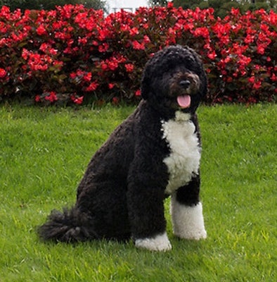
The challenge is that the pre-trained model was not trained to recognize this specific dog, and, we only have 30 pictures of Bo. If we tried to train a model from scratch using those 30 pictures we would experience overfitting and poor generalization. However, if we start with a pre-trained model that is adept at detecting dogs, we can leverage that learning to gain a generalized understanding of Bo using our smaller dataset. We can use transfer learning to solve this challenge.
Downloading the Pretrained Model
The ImageNet pre-trained models are often good choices for computer vision transfer learning, as they have learned to classify various different types of images. In doing this, they have learned to detect many different types of features that could be valuable in image recognition. Because ImageNet models have learned to detect animals, including dogs, it is especially well suited for this transfer learning task of detecting Bo.
Let us start by downloading the pre-trained model. Again, this is available directly from the Keras library. As we are downloading, there is going to be an important difference. The last layer of an ImageNet model is a dense layer of 1000 units, representing the 1000 possible classes in the dataset. In our case, we want it to make a different classification: is this Bo or not? Because we want the classification to be different, we are going to remove the last layer of the model. We can do this by setting the flag include_top=False when downloading the model. After removing this top layer, we can add new layers that will yield the type of classification that we want:
from tensorflow import keras

base_model = keras.applications.VGG16(
    weights='imagenet',  # Load weights pre-trained on ImageNet.
    input_shape=(224, 224, 3),
    include_top=False)
base_model.summary()
Model: "vgg16"
_________________________________________________________________
 Layer (type)                Output Shape              Param #
=================================================================
 input_1 (InputLayer)        [(None, 224, 224, 3)]     0

 block1_conv1 (Conv2D)       (None, 224, 224, 64)      1792

 block1_conv2 (Conv2D)       (None, 224, 224, 64)      36928

 block1_pool (MaxPooling2D)  (None, 112, 112, 64)      0

 block2_conv1 (Conv2D)       (None, 112, 112, 128)     73856

 block2_conv2 (Conv2D)       (None, 112, 112, 128)     147584

 block2_pool (MaxPooling2D)  (None, 56, 56, 128)       0

 block3_conv1 (Conv2D)       (None, 56, 56, 256)       295168

 block3_conv2 (Conv2D)       (None, 56, 56, 256)       590080

 block3_conv3 (Conv2D)       (None, 56, 56, 256)       590080

 block3_pool (MaxPooling2D)  (None, 28, 28, 256)       0

 block4_conv1 (Conv2D)       (None, 28, 28, 512)       1180160

 block4_conv2 (Conv2D)       (None, 28, 28, 512)       2359808

 block4_conv3 (Conv2D)       (None, 28, 28, 512)       2359808

 block4_pool (MaxPooling2D)  (None, 14, 14, 512)       0

 block5_conv1 (Conv2D)       (None, 14, 14, 512)       2359808

 block5_conv2 (Conv2D)       (None, 14, 14, 512)       2359808

 block5_conv3 (Conv2D)       (None, 14, 14, 512)       2359808

 block5_pool (MaxPooling2D)  (None, 7, 7, 512)         0

=================================================================
Total params: 14,714,688
Trainable params: 14,714,688
Non-trainable params: 0
_________________________________________________________________
Freezing the Base Model
Before we add our new layers onto the pre-trained model, we should take an important step: freezing the model’s pre-trained layers. This means that when we train, we will not update the base layers from the pre-trained model. Instead we will only update the new layers that we add on the end for our new classification. We freeze the initial layers because we want to retain the learning achieved from training on the ImageNet dataset. If they were unfrozen at this stage, we would likely destroy this valuable information. There will be an option to unfreeze and train these layers later, in a process called fine-tuning.
Freezing the base layers is as simple as setting trainable on the model to False.
base_model.trainable = False
Adding New Layers
We can now add the new trainable layers to the pre-trained model. They will take the features from the pre-trained layers and turn them into predictions on the new dataset. We will add two layers to the model. First will be a pooling layer like we saw in our earlier convolutional neural network. (If you want a more thorough understanding of the role of pooling layers in CNNs, please read this detailed blog post). We then need to add our final layer, which will classify Bo or not Bo. This will be a densely connected layer with one output.
inputs = keras.Input(shape=(224, 224, 3))
# Separately from setting trainable on the model, we set training to False
x = base_model(inputs, training=False)
x = keras.layers.GlobalAveragePooling2D()(x)
# A Dense classifier with a single unit (binary classification)
outputs = keras.layers.Dense(1)(x)
model = keras.Model(inputs, outputs)
type(base_model)
keras.engine.functional.Functional
Let us take a look at the model, now that we have combined the pre-trained model with the new layers.
model.summary()
Model: "model"
_________________________________________________________________
 Layer (type)                Output Shape              Param #
=================================================================
 input_2 (InputLayer)        [(None, 224, 224, 3)]     0

 vgg16 (Functional)          (None, 7, 7, 512)         14714688

 global_average_pooling2d (G  (None, 512)              0
 lobalAveragePooling2D)

 dense (Dense)               (None, 1)                 513

=================================================================
Total params: 14,715,201
Trainable params: 513
Non-trainable params: 14,714,688
_________________________________________________________________
Keras gives us a nice summary here, as it shows the vgg16 pre-trained model as one unit, rather than showing all of the internal layers. It is also worth noting that we have many non-trainable parameters as we have frozen the pre-trained model.
Compiling the Model
As with our previous exercises, we need to compile the model with loss and metrics options. We have to make some different choices here. In previous cases we had many categories in our classification problem. As a result, we picked categorical crossentropy for the calculation of our loss. In this case we only have a binary classification problem (Bo or not Bo), and so we will use binary crossentropy. Further detail about the differences between the two can found here. We will also use binary accuracy instead of traditional accuracy.
By setting from_logits=True we inform the loss function that the output values are not normalized (e.g. with softmax).
# Important to use binary crossentropy and binary accuracy as we now have a binary classification problem
model.compile(loss=keras.losses.BinaryCrossentropy(from_logits=True), metrics=[keras.metrics.BinaryAccuracy()])
Augmenting the Data
Now that we are dealing with a very small dataset, it is especially important that we augment our data. As before, we will make small modifications to the existing images, which will allow the model to see a wider variety of images to learn from. This will help it learn to recognize new pictures of Bo instead of just memorizing the pictures it trains on.
from tensorflow.keras.preprocessing.image import ImageDataGenerator
# create a data generator
datagen = ImageDataGenerator(
        samplewise_center=True,  # set each sample mean to 0
        rotation_range=10,  # randomly rotate images in the range (degrees, 0 to 180)
        zoom_range = 0.1, # Randomly zoom image
        width_shift_range=0.1,  # randomly shift images horizontally (fraction of total width)
        height_shift_range=0.1,  # randomly shift images vertically (fraction of total height)
        horizontal_flip=True,  # randomly flip images
        vertical_flip=False) # we don't expect Bo to be upside-down so we will not flip vertically
Loading the Data
We have seen datasets in a couple different formats so far. In the MNIST exercise, we were able to download the dataset directly from within the Keras library. For the sign language dataset, the data was in CSV files. For this exercise, we are going to load images directly from folders using Keras’ flow_from_directory function. We have set up our directories to help this process go smoothly as our labels are inferred from the folder names. In the data/presidential_doggy_door directory, we have train and validation directories, which each have folders for images of Bo and not Bo. In the not_bo directories, we have pictures of other dogs and cats, to teach our model to keep out other pets. Feel free to explore the images to get a sense of our dataset.
Note that flow_from_directory will also allow us to size our images to match the model: 244x244 pixels with 3 channels.
# load and iterate training dataset
train_it = datagen.flow_from_directory('data/presidential_doggy_door/train/',
                                       target_size=(224, 224),
                                       color_mode='rgb',
                                       class_mode='binary',
                                       batch_size=8)
# load and iterate validation dataset
valid_it = datagen.flow_from_directory('data/presidential_doggy_door/valid/',
                                      target_size=(224, 224),
                                      color_mode='rgb',
                                      class_mode='binary',
                                      batch_size=8)
Found 139 images belonging to 2 classes.
Found 30 images belonging to 2 classes.
Training the Model
Time to train our model and see how it does. Recall that when using a data generator, we have to explicitly set the number of steps_per_epoch:
model.fit(train_it, steps_per_epoch=12, validation_data=valid_it, validation_steps=4, epochs=20)
Epoch 1/20
12/12 [==============================] - 10s 863ms/step - loss: 0.6587 - binary_accuracy: 0.8462 - val_loss: 1.0093 - val_binary_accuracy: 0.8000
Epoch 2/20
12/12 [==============================] - 10s 866ms/step - loss: 0.2739 - binary_accuracy: 0.9271 - val_loss: 0.7576 - val_binary_accuracy: 0.8333
Epoch 3/20
12/12 [==============================] - 10s 883ms/step - loss: 0.1999 - binary_accuracy: 0.9375 - val_loss: 0.2260 - val_binary_accuracy: 0.9333
Epoch 4/20
12/12 [==============================] - 10s 877ms/step - loss: 0.0223 - binary_accuracy: 1.0000 - val_loss: 0.3512 - val_binary_accuracy: 0.9000
Epoch 5/20
12/12 [==============================] - 10s 827ms/step - loss: 0.0345 - binary_accuracy: 0.9890 - val_loss: 0.0788 - val_binary_accuracy: 0.9667
Epoch 6/20
12/12 [==============================] - 10s 885ms/step - loss: 0.0400 - binary_accuracy: 0.9896 - val_loss: 0.5098 - val_binary_accuracy: 0.8667
Epoch 7/20
12/12 [==============================] - 10s 844ms/step - loss: 0.0212 - binary_accuracy: 0.9890 - val_loss: 0.5833 - val_binary_accuracy: 0.8667
Epoch 8/20
12/12 [==============================] - 10s 839ms/step - loss: 0.0215 - binary_accuracy: 0.9890 - val_loss: 0.1980 - val_binary_accuracy: 0.9333
Epoch 9/20
12/12 [==============================] - 11s 892ms/step - loss: 0.0035 - binary_accuracy: 1.0000 - val_loss: 0.0081 - val_binary_accuracy: 1.0000
Epoch 10/20
12/12 [==============================] - 10s 834ms/step - loss: 0.0057 - binary_accuracy: 1.0000 - val_loss: 0.0199 - val_binary_accuracy: 1.0000
Epoch 11/20
12/12 [==============================] - 10s 840ms/step - loss: 0.0020 - binary_accuracy: 1.0000 - val_loss: 0.0705 - val_binary_accuracy: 0.9667
Epoch 12/20
12/12 [==============================] - 10s 854ms/step - loss: 0.0060 - binary_accuracy: 1.0000 - val_loss: 0.1651 - val_binary_accuracy: 0.9333
Epoch 13/20
12/12 [==============================] - 10s 868ms/step - loss: 0.0017 - binary_accuracy: 1.0000 - val_loss: 0.0191 - val_binary_accuracy: 1.0000
Epoch 14/20
12/12 [==============================] - 10s 847ms/step - loss: 6.5634e-04 - binary_accuracy: 1.0000 - val_loss: 0.1604 - val_binary_accuracy: 0.9333
Epoch 15/20
12/12 [==============================] - 10s 836ms/step - loss: 8.5303e-04 - binary_accuracy: 1.0000 - val_loss: 0.1170 - val_binary_accuracy: 0.9667
Epoch 16/20
12/12 [==============================] - 10s 834ms/step - loss: 6.4780e-04 - binary_accuracy: 1.0000 - val_loss: 0.1249 - val_binary_accuracy: 0.9667
Epoch 17/20
12/12 [==============================] - 11s 952ms/step - loss: 3.4196e-04 - binary_accuracy: 1.0000 - val_loss: 0.0075 - val_binary_accuracy: 1.0000
Epoch 18/20
12/12 [==============================] - 11s 888ms/step - loss: 2.8458e-04 - binary_accuracy: 1.0000 - val_loss: 0.0163 - val_binary_accuracy: 1.0000
Epoch 19/20
12/12 [==============================] - 10s 863ms/step - loss: 1.5362e-04 - binary_accuracy: 1.0000 - val_loss: 0.2103 - val_binary_accuracy: 0.9333
Epoch 20/20
12/12 [==============================] - 10s 878ms/step - loss: 2.1426e-04 - binary_accuracy: 1.0000 - val_loss: 0.2680 - val_binary_accuracy: 0.9333


<keras.callbacks.History at 0x16b5090d0>
Discussion of Results
Both the training and validation accuracy should be quite high. This is a pretty awesome result! We were able to train on a small dataset, but because of the knowledge transferred from the ImageNet model, it was able to achieve high accuracy and generalize well. This means it has a very good sense of Bo and pets who are not Bo.
If you saw some fluctuation in the validation accuracy, that is okay too. We have a technique for improving our model in the next section.
Fine-Tuning the Model
Now that the new layers of the model are trained, we have the option to apply a final trick to improve the model, called fine-tuning. To do this we unfreeze the entire model, and train it again with a very small learning rate. This will cause the base pre-trained layers to take very small steps and adjust slightly, improving the model by a small amount.
Note that it is important to only do this step after the model with frozen layers has been fully trained. The untrained pooling and classification layers that we added to the model earlier were randomly initialized. This means they needed to be updated quite a lot to correctly classify the images. Through the process of backpropagation, large initial updates in the last layers would have caused potentially large updates in the pre-trained layers as well. These updates would have destroyed those important pre-trained features. However, now that those final layers are trained and have converged, any updates to the model as a whole will be much smaller (especially with a very small learning rate) and will not destroy the features of the earlier layers.
Let’s try unfreezing the pre-trained layers, and then fine tuning the model:
# Unfreeze the base model
base_model.trainable = True

# It's important to recompile your model after you make any changes
# to the `trainable` attribute of any inner layer, so that your changes
# are taken into account
model.compile(optimizer=keras.optimizers.RMSprop(learning_rate = .00001),  # Very low learning rate
              loss=keras.losses.BinaryCrossentropy(from_logits=True),
              metrics=[keras.metrics.BinaryAccuracy()])
WARNING:absl:At this time, the v2.11+ optimizer `tf.keras.optimizers.RMSprop` runs slowly on M1/M2 Macs, please use the legacy Keras optimizer instead, located at `tf.keras.optimizers.legacy.RMSprop`.
WARNING:absl:There is a known slowdown when using v2.11+ Keras optimizers on M1/M2 Macs. Falling back to the legacy Keras optimizer, i.e., `tf.keras.optimizers.legacy.RMSprop`.
model.fit(train_it, steps_per_epoch=12, validation_data=valid_it, validation_steps=4, epochs=10)
Epoch 1/10
12/12 [==============================] - 29s 2s/step - loss: 0.0073 - binary_accuracy: 1.0000 - val_loss: 0.0021 - val_binary_accuracy: 1.0000
Epoch 2/10
12/12 [==============================] - 27s 2s/step - loss: 5.7280e-05 - binary_accuracy: 1.0000 - val_loss: 9.5360e-05 - val_binary_accuracy: 1.0000
Epoch 3/10
12/12 [==============================] - 28s 2s/step - loss: 6.2975e-05 - binary_accuracy: 1.0000 - val_loss: 0.0110 - val_binary_accuracy: 1.0000
Epoch 4/10
12/12 [==============================] - 27s 2s/step - loss: 4.1730e-05 - binary_accuracy: 1.0000 - val_loss: 3.9649e-04 - val_binary_accuracy: 1.0000
Epoch 5/10
12/12 [==============================] - 27s 2s/step - loss: 9.7147e-06 - binary_accuracy: 1.0000 - val_loss: 3.4843e-04 - val_binary_accuracy: 1.0000
Epoch 6/10
12/12 [==============================] - 27s 2s/step - loss: 1.1001e-05 - binary_accuracy: 1.0000 - val_loss: 7.9790e-04 - val_binary_accuracy: 1.0000
Epoch 7/10
12/12 [==============================] - 27s 2s/step - loss: 4.2412e-06 - binary_accuracy: 1.0000 - val_loss: 0.0226 - val_binary_accuracy: 1.0000
Epoch 8/10
12/12 [==============================] - 29s 2s/step - loss: 1.4322e-06 - binary_accuracy: 1.0000 - val_loss: 4.4826e-04 - val_binary_accuracy: 1.0000
Epoch 9/10
12/12 [==============================] - 27s 2s/step - loss: 2.8613e-06 - binary_accuracy: 1.0000 - val_loss: 9.0710e-06 - val_binary_accuracy: 1.0000
Epoch 10/10
12/12 [==============================] - 27s 2s/step - loss: 1.2063e-06 - binary_accuracy: 1.0000 - val_loss: 2.8605e-04 - val_binary_accuracy: 1.0000


<keras.callbacks.History at 0x16e6aee50>
Examining the Predictions
Now that we have a well-trained model, it is time to create our doggy door for Bo! We can start by looking at the predictions that come from the model. We will preprocess the image in the same way we did for our last doggy door.
import matplotlib.pyplot as plt
import matplotlib.image as mpimg
from tensorflow.keras.preprocessing import image as image_utils
from tensorflow.keras.applications.imagenet_utils import preprocess_input

def show_image(image_path):
    image = mpimg.imread(image_path)
    plt.imshow(image)

def make_predictions(image_path):
    show_image(image_path)
    image = image_utils.load_img(image_path, target_size=(224, 224))
    image = image_utils.img_to_array(image)
    image = image.reshape(1,224,224,3)
    image = preprocess_input(image)
    preds = model.predict(image)
    return preds
Try this out on a couple images to see the predictions:
make_predictions('data/presidential_doggy_door/valid/bo/bo_20.jpg')
1/1 [==============================] - 0s 157ms/step


array([[-15.519991]], dtype=float32)
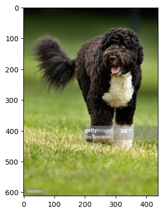
make_predictions('data/presidential_doggy_door/valid/not_bo/121.jpg')
1/1 [==============================] - 0s 156ms/step


array([[36.77488]], dtype=float32)
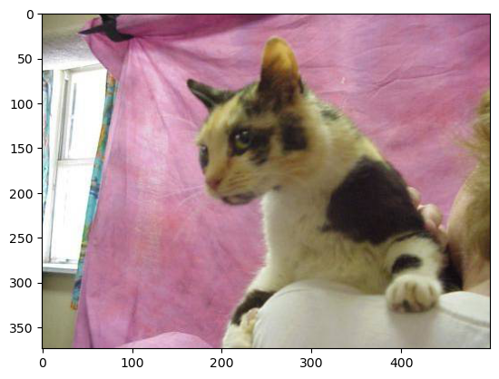
It looks like a negative number prediction means that it is Bo and a positive number prediction means it is something else. We can use this information to have our doggy door only let Bo in!
Exercise: Bo’s Doggy Door
Fill in the following code to implement Bo’s doggy door:
def presidential_doggy_door(image_path):
    preds = make_predictions(image_path)
    if preds[0] < 0:
        print("It's Bo! Let him in!")
    else:
        print("That's not Bo! Stay out!")
Let’s try it out!
presidential_doggy_door('data/presidential_doggy_door/valid/not_bo/131.jpg')
1/1 [==============================] - 0s 132ms/step
That's not Bo! Stay out!
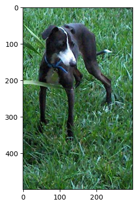
presidential_doggy_door('data/presidential_doggy_door/valid/bo/bo_29.jpg')
1/1 [==============================] - 0s 110ms/step
It's Bo! Let him in!
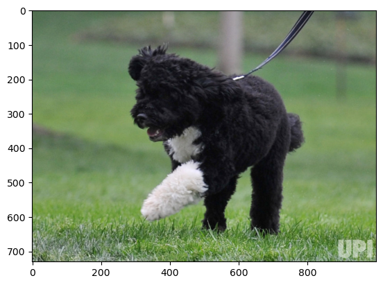
Summary
Great work! With transfer learning, you have built a highly accurate model using a very small dataset. This can be an extremely powerful technique, and be the difference between a successful project and one that cannot get off the ground. We hope these techniques can help you out in similar situations in the future!
There is a wealth of helpful resources for transfer learning in the NVIDIA TAO Toolkit.
Clear the Memory
Before moving on, please execute the following cell to clear up the GPU memory.
import IPython
app = IPython.Application.instance()
app.kernel.do_shutdown(True)
Key Points
FIX
Transferring your workflow to an HPC system
Overview
Teaching: 30 min
Exercises: 0 minQuestions
Main challenges and reasons to transition to an HPC system.
Objectives
Understand main steps related with moving to an HPC system
It is very often the case when working on machine and deep learning problems to begin prototyping in your laptop or desktop computer, but as your make progress you may soon find that the problem grows in complexity and your local hardware might not be suitable anymore. Purchasing new hardware can be prohibitive expensive and the technical details hard to understand.
One solution for these situations is to approach services like Google Colab or Amazon SageMaker which offer access to free GPU devices and can be quite attractive due to reducing the amount of hardware configuration knowledge required to start producing results.
The downside is that, as before, as your model and datasets grow, you might need the pay versions of these services to continue making progress at a suitable rate (especially when trying to meet a deadline). This option might work for expert data and machine learning scientists and practitioners who can accurately budget number of core hours and amount of storage required, but might not work as well for somebody in the model developing stages and who has started to test more challenging scenarios.
What to do in this situation? There is no simple answer, and most of the time it might be to try to adapt to what you have, but it might also be that you are a student/researcher in a university that provides you with a High Performance Computing system and that you can use it free of charge as is the case with Cardiff University’s Hawk Supercomputer.
The challenge with this solution is to adapt to a new working environment which includes learning Linux commands (in a text-based console!), concepts such as job schedulers and scripting in new languages such as Bash. Fortunately, there is also a dedicated team (Advance Research at Cardiff) that works continuously to try to make this transition as smooth as possible by offering regular training sessions on these topics for new users, solving queries when a cryptic software error occurs or any other technical challenge in the process of implementing your machine or deep learning application.
Making the transition
So, what is actually involved in this transition? For this training course we will assume that you have or are willing to request an account on the Hawk supercomputer.
As mentioned above, you will need to learn new concepts on Linux, programming on Bash and general HPC terms such as the use of job schedulers. And to put all of them together to be able to write a job script that will execute the application that you developed in your local computer or cloud service of choice. We won’t delve into the specifics of these topics since you can follow the provided links to find dedicate training courses but instead summarize the essential steps to transfer our deep learning model develop in the previous lesson to Hawk.
Exporting your Jupyter Notebook to a Python script
This is the first step in moving towards a non-interactive system and we have some advice on this respect in our Code migration to HPC systems training material. Following the advice in that link, you might end with a Python script similar to this one:
Click to expand the code
#!/usr/bin/env python
import tensorflow as tf
import matplotlib.pyplot as plt
from tensorflow.keras import models
from tensorflow.keras import layers
from tensorflow.keras.utils import to_categorical
from keras.datasets import mnist

import os
os.environ['TF_CPP_MIN_LOG_LEVEL'] = '2'

(train_images, train_labels),(test_images, test_labels) = mnist.load_data()

print("Number of train images: ", train_images.shape)
print("Number of train labels: ", train_labels.shape)
print("Number of test images: ", test_images.shape)
print("Number of test labels: ", test_labels.shape)

network = models.Sequential()
network.add(layers.Dense(512,activation='relu',input_shape=(28 * 28,)))
network.add(layers.Dense(10,activation='softmax'))

network.summary()
network.get_weights()

network.compile(optimizer='rmsprop',
                loss='categorical_crossentropy',
                metrics=['accuracy'])

train_images = train_images.reshape((60000,28 * 28))
train_images = train_images.astype('float32')/255
test_images = test_images.reshape((10000,28 * 28))
test_images = test_images.astype('float32')/255

train_labels = to_categorical(train_labels)
test_labels = to_categorical(test_labels)

network.fit(train_images,train_labels,epochs=20,batch_size=128,verbose=2)
test_loss, test_acc = network.evaluate(test_images,test_labels,verbose=2)
print('test_acc:',test_acc)
Transferring data
First, we need to be able to transfer our scripts and any data required. There are a few options to reach this goal, but we will focus on using the terminal and scp
$ scp my-script.py username@hawklogin.cf.ac.uk
The above command will transfer your script directly into your home directory in the remove server (the supercomputer Hawk). You can repeat the command to transfer any other required files. After this, we can login into the remote server to prepare things to run our application.
$ ssh username@hawklogin.cf.ac.uk
Installing software
HPC systems like Hawk usually provide a rich software environment with many useful tools. However, it might be that we have a specific working environment that we would like to replicate as is often the case when working with Anaconda and Python libraries. In this case it is useful to create a virtual environment with all the dependencies that your application requires. On Hawk you can do this with (using the environment yaml file provided for this course, check the setup section):
$ module load anaconda
$ conda env create -f environment.yml
The above command will make anaconda available in your environment to allow you to run conda to install a virtual environment called machine-learning with the packages listed in the file environment.yml. To activate the environment use:
$ conda activate machine-learning
$ (machine-learning) $ conda list
The last command above is useful to confirm that your environment has all the necessary libraries.
Writing a job script.
One of the most challenging parts of working on an HPC system like Hawk is getting used to write files know as job scripts that are simply text files with Bash commands that are executed by SLURM (a job scheduler) that decides in which order resources are allocated to users. For this training course you can use the following template (pay attention to your instructor in case modifications are required):
A very simple job script for CPUs
(Click to see the code)
#!/bin/bash
#SBATCH --job-name=ml.example
#SBATCH --error=%x.e.%J
#SBATCH --output=%x.o.%J
#SBATCH --partition=dev
#SBATCH --time=00:10:00
#SBATCH --ntasks=1
#SBATCH --account=scwXXXX

module purge
module load keras/2.3.1
module list

time python mnist-test.py
A very simple job script for GPUs
(Click to see the code)
#!/bin/bash
#SBATCH --job-name=ml.example.gpu
#SBATCH --error=%x.e.%J
#SBATCH --output=%x.o.%J
#SBATCH --partition=gpu
#SBATCH --time=00:10:00
#SBATCH --ntasks=20
#SBATCH --gres=gpu:1
#SBATCH --account=scwXXXX

module purge
module load keras/2.3.1
module list

time python mnist-test.py
A more complete job script example
(Click to see the code)
#!/bin/bash --login
#SBATCH --job-name=mnist
#SBATCH --error=%x.e.%j
#SBATCH --output=%x.o.%j
#SBATCH --partition=gpu
#SBATCH --time=00:10:00
#SBATCH --ntasks=40
#SBATCH --ntasks-per-node=40
#SBATCH --gres=gpu:2
#SBATCH --account=scwXXXX

clush -w $SLURM_NODELIST "sudo /apps/slurm/gpuset_3_exclusive"

echo '----------------------------------------------------'
echo ' NODE USED = '$SLURM_NODELIST
echo ' SLURM_JOBID = '$SLURM_JOBID
echo ' OMP_NUM_THREADS = '$OMP_NUM_THREADS
echo ' ncores = '$NP
echo ' PPN = ' $PPN
echo '----------------------------------------------------'
#
echo Running on host `hostname`
echo Time is `date`
echo Directory is `pwd`
echo SLURM job ID is $SLURM_JOBID
#
echo Number of Processing Elements is $NP
echo Number of mpiprocs per node is $PPN
env

test=mnist
input_dir=$HOME/training
WDPATH=/scratch/$USER/${test}.$SLURM_JOBID
rm -rf ${WDPATH}
mkdir -p ${WDPATH}
cd ${WDPATH}

cp ${input_dir}/${test}.py ${WDPATH}

module purge
module load anaconda
module list

source activate machine-learning

start="$(date +%s)"
time python -u -i ${test}.py
stop="$(date +%s)"
finish=$(( $stop-$start ))
echo deep learning ${test} $SLURM_JOBID Job-Time $finish seconds
echo Keras End Time is `date`
Hopefully the above script will allow recreate the examples with which we have worked in the training course.
Other challenges
We have so far used very simple test cases to demonstrate the development of machine and deep learning applications. Real world applications are more complex and new challenges are likely to appear. Two of the more common include:
- Data storage: more complex models often require huge databases that are not always simple to store even in HPC systems.
- Optimization: HPC systems tend to have high-end hardware CPU and GPU devices that often require compiling libraries with specialized settings to exploit special hardware features.
If you are having trouble with any of these issues or with any other, contact us at arcca-help@cardiff.ac.uk and we will try to help you solve it.
Key Points
Moving to an HPC system can be challenging but there are sources of help that can make the transition easier.
As you progress in the development of machine and deep learning applications new challenges are likely to appear. Requesting help in those case can save you a lot of time.