Scikit Learn - Linear Model

Overview

Teaching: 45 min
Exercises: 0 min

Questions

• Use Scikit Learn to build a simple linear regression machine learning problem.

Objectives

• Familiarize with the basic steps involved in building a machine learning model.

• Test our machine learning tools and environment.

GDP and happiness

We will start building a very simple model to predict people Happiness (as measured by the OECD) based on the country’s GDP (as provided by the IMF). This is also called model-based learning. For this course we will use Scikit-Learn but other libraries should provide similar functionalities.

Obtaining and working with data

When developing Machine Learning applications you will likely need to work with databases either by creating them yourself or obtaining some already available. Depending on the field and stage of your research, the databases can range from a few megabytes to several hundreds gigabytes and ever bigger. At that point you’ll likely need to consider carefully (even more if the database has data protection requirements) how best to manage storage requirements in order to optimize available resources in your work system. Do not hesitate to contact your system administrators to discuss further any doubts or concerns that you might have.

Luckily for this training the databases we will be working with are publicly available from the OECD’s Better Life Index) and the IMF’s GDP per capita) and only occupy a few megabytes. You can also find them in the zip file provided for this training course.

Start by loading some python libraries.

import matplotlib.pyplot as plt
import numpy as np
import pandas as pd
import sklearn.linear_model

Continue by loading the data as Pandas dataframes. For this you need to provide the corresponding file locations, for example:

file_gdp="gdp-bli/gdp_per_capita_2014-2025.csv"
file_happy="gdp-bli/BLI_25112020150937807.csv"

df_gdp=pd.read_csv(file_gdp,thousands=',',delimiter='\t',encoding='latin1',na_values='n/a')
df_happy=pd.read_csv(file_happy,thousands=',')

You can take a look at the data we just loaded with the head dataframe function, for example, to print the first 5 rows in the GDP dataframe:

rows=5
df_gdp.head(rows)

Preparing our data

Next we define a few helper functions to extract subsets of our dataset.

OECD Better Life Index dataset

The following function extracts data based on an indicator and an inequality group and then returns a dataframe with the indicator data per country:

def oecd_bli_indicator(data,indicator):
    """
    Process OECD Better Life Index data
    Extract a specific "Indicator" from the dataset
    Each indicator in the dataset is aggregated to take into
    account the inequalities of different population groups:
    
    "MN"  - Men
    "WMN" - Women
    "HGH" - High socio-economic status
    "LW"  - Low socio-economic status
    "TOT" - All population
    
    We use TOT in this example, but feel free to check the
    results with different groups.
    """
    assert indicator in data["Indicator"].unique(), "{} is not available in dataset".format(indicator)
    
    result = data[(data["INEQUALITY"]=="TOT") & (data["Indicator"]==indicator)][["Country","Value"]]
    result = result.rename(columns={"Value":indicator})
    result = result.set_index("Country").sort_values(by=["Country"])

    return result

In this example we use Life satisfaction as indicator and Total as inequality group, but feel free to try other parameters.

indicator = "Life satisfaction"
inequality = "MN"
bli_data = oecd_bli_indicator(df_happy,indicator,inequality)

Gross Domestic Product dataset from the International Monetary Fund

The function below simply selects a column from the dataset corresponding to a year and returns a dataframe with GDP information per country for that year.

def gdp_extract_year(data,year):
    """
    Process Gross Domestic Product data from IMF
    Extract data column corresponding to a specific year
    rename column and set a new index
    """
    assert year in data.columns, "{} is not available in dataset".format(year)
    gdp_year = data[["Country",year]]
    gdp_year = gdp_year.rename(columns={year:"GDP per capita {}".format(year)})
    gdp_year = gdp_year.set_index("Country")
    return gdp_year

In this example we work with year 2020, but try with other years and check if you obtain similar results.

year = "2020"
gdp_data = gdp_extract_year(df_gdp,year)

Merging our datasets

With our datasets ready, the next step is merging them based on country name. The function below is in charge of this:

def merge_by_country(gdp_data,bli_data):
    """
    Merge both datasets by country.
    We only keep those countries common to both datasets
    """
    merged_data = pd.merge(left=bli_data, right=gdp_data,left_index=True, right_index=True)
    return merged_data

Note that not all countries appear in both datasets and we only keep information for countries common to both datasets. This produces our final input dataset.

input_data = merge_by_country(gdp_data,bli_data)

Split training and testing datasets

To divide our input data in two sets for training and testing we can use Scikit Learn function train_test_split as in the previous lesson.

x_training, x_testing, y_training, y_testing = train_test_split(input_data["GDP per capita {}".format(year)].to_numpy(),
                                                                input_data["Life satisfaction"].to_numpy(),
                                                                test_size=0.25, random_state=0)

Visualising our data

Before building our model, it can be useful to visualise the data to gain insights about what type of models could be better suited for it. For this we can use the helper function below, which is prepared to plot both training and testing datasets, and a regression line using a slope (m) and intercept (b) coefficients, if provided.

import matplotlib.pyplot as plt
def scatter_plot(x_train,y_train,x_test=None,y_test=None,m=None,b=None):
    #plot training data
    plt.scatter(x_train,y_train,color='red')

    # plot testing data if given
    if (x_test is not None) and (y_test is not None):
        plt.scatter(x_test,y_test,color='green')
    
    # plot model's predicted line if coefficients given
    if (m is not None) and (b is not None):
        x = np.arange(0,100000)
        plt.plot(x, b + m * x, '-')

    plt.xlabel("GDP per capita (2020)")
    plt.ylabel("Life satisfaction")
    plt.xlim([0,100000])
    plt.ylim([0,10])

We can test our function by plotting the training dataset:

scatter_plot(x_training,y_training)

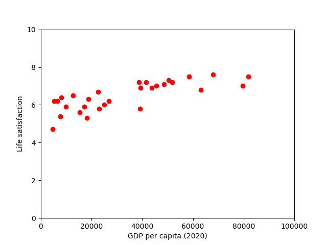
There does seem to be a trend here! Although the data is noisy (i.e., partly random), it looks like life satisfaction goes up more or less linearly as the country’s GDP per capita increases. So we decide to model life satisfaction as a linear function of GDP per capita.

Building the model

Based on the above observations, we select a linear model of life satisfaction with just one attribute, GDP per capita:

model = sklearn.linear_model.LinearRegression()

With the model selected, the next step is to fit it to the data. The calculations performed in this step are model dependent, for example, for a linear model it involves calculating a set of coefficients to minimize the residual sum of squares between the observed targets in the dataset, and the targets predicted by the linear approximation.

model.fit(np.c_[x_training], np.c_[y_training])

And we can access the estimated value for the model key parameters (which parameters are available also depends on the selected model).

print(f"model's intercept: {model.intercept_[0]}")
print(f"model's slope    : {model.coef_[0][0]}")

model's intercept: 5.77342747430831
model's slope    : 2.025726170863078e-05

It might be useful to plot our model alongside our data, including the trend line:

scatter_plot(x_training,y_training,
            m=model.coef_[0][0],b=model.intercept_[0])

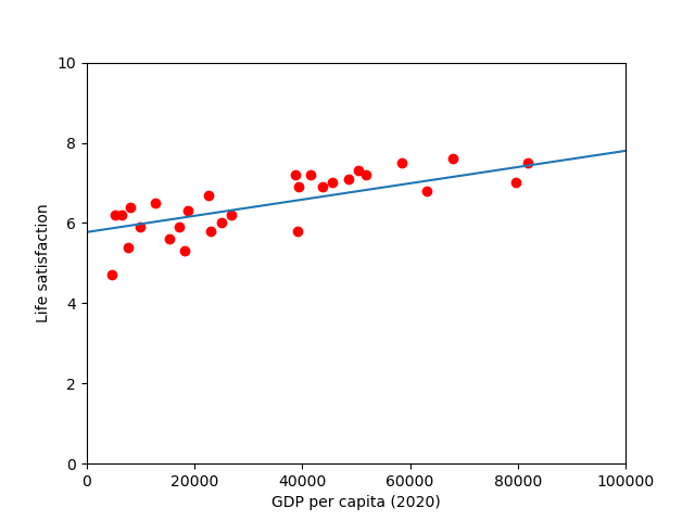
there seems to be a good fit between the training data and the trend line predicted by the model, however, we still need to compare with out test dataset.

Validating and making predictions

After we have trained our model, we should perform some validation checks using the labelled data we saved for this purpose:

model.score(np.c_[x_testing],np.c_[y_testing])

0.5010135842893668

Always helpful to have some visual aids to compare how well our model does against the validation data

scatter_plot(x_training,y_training,
             x_testing,y_testing,
             model.coef_[0][0],model.intercept_[0])

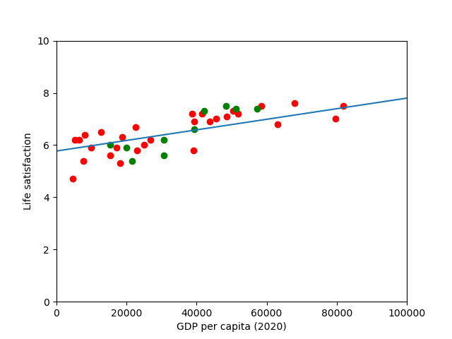
Visually, it appears as like our model is reasonably good at predicting values in our test dataset, however, a coefficient of determination of 0.50 might not be great depending on the field. At this point it might be worth thinking about using alternative indicators (employment rate, health, air) or additional features to improve our model if needed.

Key Points

• Python is a very useful programming language to develop machine learning applications

• Scikit Learn together with Numpy, Pandas and Matplotlib form a popular machine learning environment.

• Linear regression is one of the most simple and useful machine learning algorithms in which the model makes a prediction by simply computing a weighted sum of the input features, plus a constant called the intercept term.