Pretrained models & Transfer Learning
Overview
Teaching: 30 min
Exercises: 0 minQuestions
FIX
Objectives
Use Keras to load a very well-trained pretrained model
Preprocess your own images to work with the pretrained model
Use the pretrained model to perform accurate inference on your own images
Prepare a pretrained model for transfer learning
Perform transfer learning with your own small dataset on a pretrained model
Further fine tune the model for even better performance
This section is taken from NVIDIA’s Deep Learning Institute workshop: “Getting started with Deep Learning”. You can find the complete course and many others at https://www.nvidia.com/en-gb/training/online/. Please note that you may need to pay for some of these courses but ask your local DLI ambassador for a promo code to get access for free.
Pre-Trained Models
Though it is often necessary to have a large, well annotated dataset to solve a deep learning challenge, there are many freely available pre-trained models that we can use right out of the box. As you decide to take on your own deep learning project, it is a great idea to start by looking for existing models online that can help you achieve your goal. A great place to explore available models is NGC. There are also many models hosted on GitHub that you can find through searching on Google.
Objectives
- Use Keras to load a very well-trained pretrained model
- Preprocess your own images to work with the pretrained model
- Use the pretrained model to perform accurate inference on your own images
An Automated Doggy Door
In this section, we will be creating a doggy door that only lets dogs (and not other animals) in and out. We can keep our cats inside, and other animals outside where they belong. Using the techniques covered so far, we would need a very large dataset with pictures of many dogs, as well as other animals. Luckily, there is a readily available model that has been trained on a massive dataset, including lots of animals.
The ImageNet challenge has produced many state-of-the-art models that can be used for image classification. They are trained on millions of images, and can accurately classify images into 1000 different categories. Many of those categories are animals, including breeds of dogs and cats. This is a perfect model for our doggy door.
Loading the Model
We will start by downloading the model. Trained ImageNet models are available to download directly within the Keras library. You can see the available models and their details here. Any of these models would work for our exercise. We will pick a commonly used one called VGG16:
from tensorflow.keras.applications import VGG16

# load the VGG16 network *pre-trained* on the ImageNet dataset
model = VGG16(weights="imagenet")
Now that it is loaded, let us take a look at the model. It looks a lot like our convolutional model from the sign language exercise. Pay attention to the first layer (the input layer) and the last layer (the output layer). As with our earlier exercises, we need to make sure our images match the input dimensions that the model expects. It is also valuable to understand what the model will return from the final output layer.
model.summary()
Model: "vgg16"
_________________________________________________________________
 Layer (type)                Output Shape              Param #
=================================================================
 input_1 (InputLayer)        [(None, 224, 224, 3)]     0

 block1_conv1 (Conv2D)       (None, 224, 224, 64)      1792

 block1_conv2 (Conv2D)       (None, 224, 224, 64)      36928

 block1_pool (MaxPooling2D)  (None, 112, 112, 64)      0

 block2_conv1 (Conv2D)       (None, 112, 112, 128)     73856

 block2_conv2 (Conv2D)       (None, 112, 112, 128)     147584

 block2_pool (MaxPooling2D)  (None, 56, 56, 128)       0

 block3_conv1 (Conv2D)       (None, 56, 56, 256)       295168

 block3_conv2 (Conv2D)       (None, 56, 56, 256)       590080

 block3_conv3 (Conv2D)       (None, 56, 56, 256)       590080

 block3_pool (MaxPooling2D)  (None, 28, 28, 256)       0

 block4_conv1 (Conv2D)       (None, 28, 28, 512)       1180160

 block4_conv2 (Conv2D)       (None, 28, 28, 512)       2359808

 block4_conv3 (Conv2D)       (None, 28, 28, 512)       2359808

 block4_pool (MaxPooling2D)  (None, 14, 14, 512)       0

 block5_conv1 (Conv2D)       (None, 14, 14, 512)       2359808

 block5_conv2 (Conv2D)       (None, 14, 14, 512)       2359808

 block5_conv3 (Conv2D)       (None, 14, 14, 512)       2359808

 block5_pool (MaxPooling2D)  (None, 7, 7, 512)         0

 flatten (Flatten)           (None, 25088)             0

 fc1 (Dense)                 (None, 4096)              102764544

 fc2 (Dense)                 (None, 4096)              16781312

 predictions (Dense)         (None, 1000)              4097000

=================================================================
Total params: 138,357,544
Trainable params: 138,357,544
Non-trainable params: 0
_________________________________________________________________
Input dimensions
We can see that the model is expecting images in the shape of (224, 224, 3) corresponding to 224 pixels high, 224 pixels wide, and 3 color channels. As we learned in our last exercise, Keras models can accept more than one image at a time for prediction. If we pass in just one image, the shape will be (1, 224, 224, 3). We will need to make sure that when passing images into our model for prediction, they match these dimensions.
Output dimensions
We can also see that the model will return a prediction of shape 1000. Remember that in our first exercise the output shape of our model was 10, corresponding to the 10 different digits. In our second exercise we had a shape of 24, corresponding to the 24 letters of the sign language alphabet that could be captured in a still image. Here, we have 1000 possible categories that the image will be placed in. Though the full ImageNet dataset has over 20,000 categories, the competition and result in pre-trained models just use a subset of 1000 of these categories. We can take a look at all of these possible categories here.
Many of the categories are animals, including many types of dogs and cats. The dogs are categories 151 through 268. The cats are categories 281 through 285. We will be able to use these categories to tell our doggy door what type of animal is at our door, and whether we should let them in or not.
Loading an Image
We will start by loading in an image and displaying it, as we have done in previous exercises.
import matplotlib.pyplot as plt
import matplotlib.image as mpimg

def show_image(image_path):
    image = mpimg.imread(image_path)
    print(image.shape)
    plt.imshow(image)
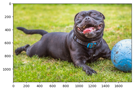
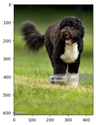
show_image("data/doggy_door_images/happy_dog.jpg")
(1200, 1800, 3)
Preprocessing the Image
Next, we need to preprocess the image so that it is ready to be sent into the model. This is just like what we did in our last exercise when we predicted on the sign language images. Remember that in this case, the final shape of the image needs to be (1, 224, 224, 3).
When loading models directly with Keras, we can also take advantage of preprocess_input methods. These methods, associated with a specific model, allow users to preprocess their own images to match the qualities of the images that the model was originally trained on. We had to do this manually yourself when performing inference with new ASL images:
from tensorflow.keras.preprocessing import image as image_utils
from tensorflow.keras.applications.vgg16 import preprocess_input

def load_and_process_image(image_path):
    # Print image's original shape, for reference
    print('Original image shape: ', mpimg.imread(image_path).shape)

    # Load in the image with a target size of 224, 224
    image = image_utils.load_img(image_path, target_size=(224, 224))
    # Convert the image from a PIL format to a numpy array
    image = image_utils.img_to_array(image)
    # Add a dimension for number of images, in our case 1
    image = image.reshape(1,224,224,3)
    # Preprocess image to align with original ImageNet dataset
    image = preprocess_input(image)
    # Print image's shape after processing
    print('Processed image shape: ', image.shape)
    return image
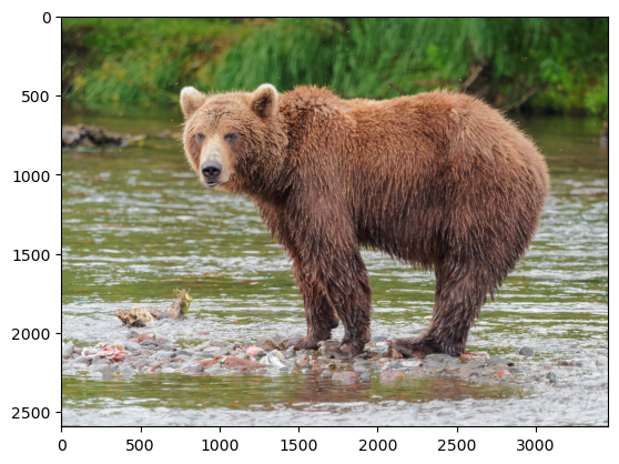
processed_image = load_and_process_image("data/doggy_door_images/brown_bear.jpg")
Original image shape:  (2592, 3456, 3)
Processed image shape:  (1, 224, 224, 3)
Make a Prediction
Now that we have our image in the right format, we can pass it into our model and get a prediction. We are expecting an output of an array of 1000 elements, which is going to be difficult to read. Fortunately, models loaded directly with Keras have yet another helpful method that will translate that prediction array into a more readable form.
from tensorflow.keras.applications.vgg16 import decode_predictions

def readable_prediction(image_path):
    # Show image
    show_image(image_path)
    # Load and pre-process image
    image = load_and_process_image(image_path)
    # Make predictions
    predictions = model.predict(image)
    # Print predictions in readable form
    print('Predicted:', decode_predictions(predictions, top=3))
Try it out on a few animals to see the results! Also feel free to upload your own images and categorize them just to see how well it works.
readable_prediction("data/doggy_door_images/happy_dog.jpg")
(1200, 1800, 3)
Original image shape:  (1200, 1800, 3)
Processed image shape:  (1, 224, 224, 3)
1/1 [==============================] - 0s 129ms/step
Downloading data from https://storage.googleapis.com/download.tensorflow.org/data/imagenet_class_index.json
35363/35363 [==============================] - 0s 1us/step
Predicted: [[('n02093256', 'Staffordshire_bullterrier', 0.4509814), ('n02110958', 'pug', 0.32263216), ('n02099712', 'Labrador_retriever', 0.09343193)]]

readable_prediction("data/doggy_door_images/brown_bear.jpg")
(2592, 3456, 3)
Original image shape:  (2592, 3456, 3)
Processed image shape:  (1, 224, 224, 3)
1/1 [==============================] - 0s 111ms/step
Predicted: [[('n02132136', 'brown_bear', 0.98538613), ('n02133161', 'American_black_bear', 0.01387624), ('n02410509', 'bison', 0.000266038)]]

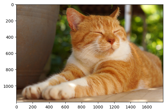
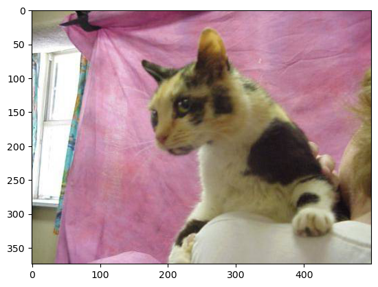
readable_prediction("data/doggy_door_images/sleepy_cat.jpg")
(1200, 1800, 3)
Original image shape:  (1200, 1800, 3)
Processed image shape:  (1, 224, 224, 3)
1/1 [==============================] - 0s 122ms/step
Predicted: [[('n02123159', 'tiger_cat', 0.7365469), ('n02124075', 'Egyptian_cat', 0.17492704), ('n02123045', 'tabby', 0.04588393)]]

Only Dogs
Now that we are making predictions with our model, we can use our categories to only let dogs in and out and keep cats inside. Remember that dogs are categories 151 through 268 and cats are categories 281 through 285. The np.argmax function can find which element of the prediction array is the top category.
import numpy as np

def doggy_door(image_path):
    show_image(image_path)
    image = load_and_process_image(image_path)
    preds = model.predict(image)
    if 151 <= np.argmax(preds) <= 268:
        print("Doggy come on in!")
    elif 281 <= np.argmax(preds) <= 285:
        print("Kitty stay inside!")
    else:
        print("You're not a dog! Stay outside!")
doggy_door("data/doggy_door_images/brown_bear.jpg")
(2592, 3456, 3)
Original image shape:  (2592, 3456, 3)
Processed image shape:  (1, 224, 224, 3)


2023-10-16 12:28:22.055577: W tensorflow/tsl/platform/profile_utils/cpu_utils.cc:128] Failed to get CPU frequency: 0 Hz


1/1 [==============================] - 0s 250ms/step
You're not a dog! Stay outside!
doggy_door("data/doggy_door_images/happy_dog.jpg")
(1200, 1800, 3)
Original image shape:  (1200, 1800, 3)
Processed image shape:  (1, 224, 224, 3)
1/1 [==============================] - 0s 117ms/step
Doggy come on in!

doggy_door("data/doggy_door_images/sleepy_cat.jpg")
(1200, 1800, 3)
Original image shape:  (1200, 1800, 3)
Processed image shape:  (1, 224, 224, 3)
1/1 [==============================] - 0s 113ms/step
Kitty stay inside!
Summary
Great work! Using a powerful pre-trained model, we have created a functional doggy door in just a few lines of code. We hope you are excited to realize that you can take advantage of deep learning without a lot of up-front work. The best part is, as the deep learning community moves forward, more models will become available for you to use on your own projects.
Clear the Memory
Before moving on, please execute the following cell to clear up the GPU memory.
import IPython
app = IPython.Application.instance()
app.kernel.do_shutdown(True)
Next
Using pretrained models is incredibly powerful, but sometimes they are not a perfect fit for your data. In the next section you will learn about another powerful technique, transfer learning, which allows you to tailer pretrained models to make good predictions for your data.
Transfer Learning
So far, we have trained accurate models on large datasets, and also downloaded a pre-trained model that we used with no training necessary. But what if we cannot find a pre-trained model that does exactly what you need, and what if we do not have a sufficiently large dataset to train a model from scratch? In this case, there is a very helpful technique we can use called transfer learning.
With transfer learning, we take a pre-trained model and retrain it on a task that has some overlap with the original training task. A good analogy for this is an artist who is skilled in one medium, such as painting, who wants to learn to practice in another medium, such as charcoal drawing. We can imagine that the skills they learned while painting would be very valuable in learning how to draw with charcoal.
As an example in deep learning, say we have a pre-trained model that is very good at recognizing different types of cars, and we want to train a model to recognize types of motorcycles. A lot of the learnings of the car model would likely be very useful, for instance the ability to recognize headlights and wheels.
Transfer learning is especially powerful when we do not have a large and varied dataset. In this case, a model trained from scratch would likely memorize the training data quickly, but not be able to generalize well to new data. With transfer learning, you can increase your chances of training an accurate and robust model on a small dataset.
Objectives
- Prepare a pretrained model for transfer learning
- Perform transfer learning with your own small dataset on a pretrained model
- Further fine tune the model for even better performance
A Personalized Doggy Door
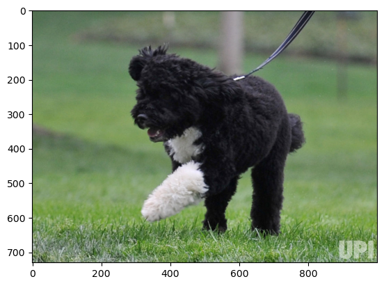
In our last exercise, we used a pre-trained ImageNet model to let in all dogs, but keep out other animals. In this exercise, we would like to create a doggy door that only lets in a particular dog. In this case, we will make an automatic doggy door for a dog named Bo, the United States First Dog between 2009 and 2017. There are more pictures of Bo in the data/presidential_doggy_door folder.
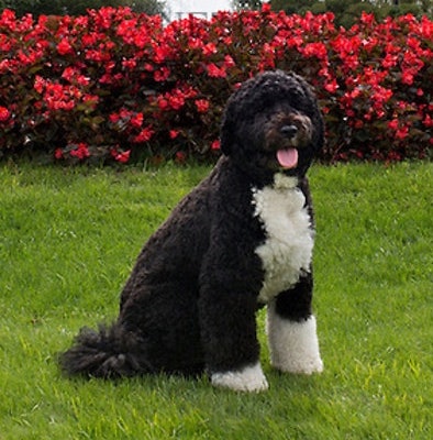
The challenge is that the pre-trained model was not trained to recognize this specific dog, and, we only have 30 pictures of Bo. If we tried to train a model from scratch using those 30 pictures we would experience overfitting and poor generalization. However, if we start with a pre-trained model that is adept at detecting dogs, we can leverage that learning to gain a generalized understanding of Bo using our smaller dataset. We can use transfer learning to solve this challenge.
Downloading the Pretrained Model
The ImageNet pre-trained models are often good choices for computer vision transfer learning, as they have learned to classify various different types of images. In doing this, they have learned to detect many different types of features that could be valuable in image recognition. Because ImageNet models have learned to detect animals, including dogs, it is especially well suited for this transfer learning task of detecting Bo.
Let us start by downloading the pre-trained model. Again, this is available directly from the Keras library. As we are downloading, there is going to be an important difference. The last layer of an ImageNet model is a dense layer of 1000 units, representing the 1000 possible classes in the dataset. In our case, we want it to make a different classification: is this Bo or not? Because we want the classification to be different, we are going to remove the last layer of the model. We can do this by setting the flag include_top=False when downloading the model. After removing this top layer, we can add new layers that will yield the type of classification that we want:
from tensorflow import keras

base_model = keras.applications.VGG16(
    weights='imagenet',  # Load weights pre-trained on ImageNet.
    input_shape=(224, 224, 3),
    include_top=False)
base_model.summary()
Model: "vgg16"
_________________________________________________________________
 Layer (type)                Output Shape              Param #
=================================================================
 input_1 (InputLayer)        [(None, 224, 224, 3)]     0

 block1_conv1 (Conv2D)       (None, 224, 224, 64)      1792

 block1_conv2 (Conv2D)       (None, 224, 224, 64)      36928

 block1_pool (MaxPooling2D)  (None, 112, 112, 64)      0

 block2_conv1 (Conv2D)       (None, 112, 112, 128)     73856

 block2_conv2 (Conv2D)       (None, 112, 112, 128)     147584

 block2_pool (MaxPooling2D)  (None, 56, 56, 128)       0

 block3_conv1 (Conv2D)       (None, 56, 56, 256)       295168

 block3_conv2 (Conv2D)       (None, 56, 56, 256)       590080

 block3_conv3 (Conv2D)       (None, 56, 56, 256)       590080

 block3_pool (MaxPooling2D)  (None, 28, 28, 256)       0

 block4_conv1 (Conv2D)       (None, 28, 28, 512)       1180160

 block4_conv2 (Conv2D)       (None, 28, 28, 512)       2359808

 block4_conv3 (Conv2D)       (None, 28, 28, 512)       2359808

 block4_pool (MaxPooling2D)  (None, 14, 14, 512)       0

 block5_conv1 (Conv2D)       (None, 14, 14, 512)       2359808

 block5_conv2 (Conv2D)       (None, 14, 14, 512)       2359808

 block5_conv3 (Conv2D)       (None, 14, 14, 512)       2359808

 block5_pool (MaxPooling2D)  (None, 7, 7, 512)         0

=================================================================
Total params: 14,714,688
Trainable params: 14,714,688
Non-trainable params: 0
_________________________________________________________________
Freezing the Base Model
Before we add our new layers onto the pre-trained model, we should take an important step: freezing the model’s pre-trained layers. This means that when we train, we will not update the base layers from the pre-trained model. Instead we will only update the new layers that we add on the end for our new classification. We freeze the initial layers because we want to retain the learning achieved from training on the ImageNet dataset. If they were unfrozen at this stage, we would likely destroy this valuable information. There will be an option to unfreeze and train these layers later, in a process called fine-tuning.
Freezing the base layers is as simple as setting trainable on the model to False.
base_model.trainable = False
Adding New Layers
We can now add the new trainable layers to the pre-trained model. They will take the features from the pre-trained layers and turn them into predictions on the new dataset. We will add two layers to the model. First will be a pooling layer like we saw in our earlier convolutional neural network. (If you want a more thorough understanding of the role of pooling layers in CNNs, please read this detailed blog post). We then need to add our final layer, which will classify Bo or not Bo. This will be a densely connected layer with one output.
inputs = keras.Input(shape=(224, 224, 3))
# Separately from setting trainable on the model, we set training to False
x = base_model(inputs, training=False)
x = keras.layers.GlobalAveragePooling2D()(x)
# A Dense classifier with a single unit (binary classification)
outputs = keras.layers.Dense(1)(x)
model = keras.Model(inputs, outputs)
type(base_model)
keras.engine.functional.Functional
Let us take a look at the model, now that we have combined the pre-trained model with the new layers.
model.summary()
Model: "model"
_________________________________________________________________
 Layer (type)                Output Shape              Param #
=================================================================
 input_2 (InputLayer)        [(None, 224, 224, 3)]     0

 vgg16 (Functional)          (None, 7, 7, 512)         14714688

 global_average_pooling2d (G  (None, 512)              0
 lobalAveragePooling2D)

 dense (Dense)               (None, 1)                 513

=================================================================
Total params: 14,715,201
Trainable params: 513
Non-trainable params: 14,714,688
_________________________________________________________________
Keras gives us a nice summary here, as it shows the vgg16 pre-trained model as one unit, rather than showing all of the internal layers. It is also worth noting that we have many non-trainable parameters as we have frozen the pre-trained model.
Compiling the Model
As with our previous exercises, we need to compile the model with loss and metrics options. We have to make some different choices here. In previous cases we had many categories in our classification problem. As a result, we picked categorical crossentropy for the calculation of our loss. In this case we only have a binary classification problem (Bo or not Bo), and so we will use binary crossentropy. Further detail about the differences between the two can found here. We will also use binary accuracy instead of traditional accuracy.
By setting from_logits=True we inform the loss function that the output values are not normalized (e.g. with softmax).
# Important to use binary crossentropy and binary accuracy as we now have a binary classification problem
model.compile(loss=keras.losses.BinaryCrossentropy(from_logits=True), metrics=[keras.metrics.BinaryAccuracy()])
Augmenting the Data
Now that we are dealing with a very small dataset, it is especially important that we augment our data. As before, we will make small modifications to the existing images, which will allow the model to see a wider variety of images to learn from. This will help it learn to recognize new pictures of Bo instead of just memorizing the pictures it trains on.
from tensorflow.keras.preprocessing.image import ImageDataGenerator
# create a data generator
datagen = ImageDataGenerator(
        samplewise_center=True,  # set each sample mean to 0
        rotation_range=10,  # randomly rotate images in the range (degrees, 0 to 180)
        zoom_range = 0.1, # Randomly zoom image
        width_shift_range=0.1,  # randomly shift images horizontally (fraction of total width)
        height_shift_range=0.1,  # randomly shift images vertically (fraction of total height)
        horizontal_flip=True,  # randomly flip images
        vertical_flip=False) # we don't expect Bo to be upside-down so we will not flip vertically
Loading the Data
We have seen datasets in a couple different formats so far. In the MNIST exercise, we were able to download the dataset directly from within the Keras library. For the sign language dataset, the data was in CSV files. For this exercise, we are going to load images directly from folders using Keras’ flow_from_directory function. We have set up our directories to help this process go smoothly as our labels are inferred from the folder names. In the data/presidential_doggy_door directory, we have train and validation directories, which each have folders for images of Bo and not Bo. In the not_bo directories, we have pictures of other dogs and cats, to teach our model to keep out other pets. Feel free to explore the images to get a sense of our dataset.
Note that flow_from_directory will also allow us to size our images to match the model: 244x244 pixels with 3 channels.
# load and iterate training dataset
train_it = datagen.flow_from_directory('data/presidential_doggy_door/train/',
                                       target_size=(224, 224),
                                       color_mode='rgb',
                                       class_mode='binary',
                                       batch_size=8)
# load and iterate validation dataset
valid_it = datagen.flow_from_directory('data/presidential_doggy_door/valid/',
                                      target_size=(224, 224),
                                      color_mode='rgb',
                                      class_mode='binary',
                                      batch_size=8)
Found 139 images belonging to 2 classes.
Found 30 images belonging to 2 classes.
Training the Model
Time to train our model and see how it does. Recall that when using a data generator, we have to explicitly set the number of steps_per_epoch:
model.fit(train_it, steps_per_epoch=12, validation_data=valid_it, validation_steps=4, epochs=20)
Epoch 1/20
12/12 [==============================] - 10s 863ms/step - loss: 0.6587 - binary_accuracy: 0.8462 - val_loss: 1.0093 - val_binary_accuracy: 0.8000
Epoch 2/20
12/12 [==============================] - 10s 866ms/step - loss: 0.2739 - binary_accuracy: 0.9271 - val_loss: 0.7576 - val_binary_accuracy: 0.8333
Epoch 3/20
12/12 [==============================] - 10s 883ms/step - loss: 0.1999 - binary_accuracy: 0.9375 - val_loss: 0.2260 - val_binary_accuracy: 0.9333
Epoch 4/20
12/12 [==============================] - 10s 877ms/step - loss: 0.0223 - binary_accuracy: 1.0000 - val_loss: 0.3512 - val_binary_accuracy: 0.9000
Epoch 5/20
12/12 [==============================] - 10s 827ms/step - loss: 0.0345 - binary_accuracy: 0.9890 - val_loss: 0.0788 - val_binary_accuracy: 0.9667
Epoch 6/20
12/12 [==============================] - 10s 885ms/step - loss: 0.0400 - binary_accuracy: 0.9896 - val_loss: 0.5098 - val_binary_accuracy: 0.8667
Epoch 7/20
12/12 [==============================] - 10s 844ms/step - loss: 0.0212 - binary_accuracy: 0.9890 - val_loss: 0.5833 - val_binary_accuracy: 0.8667
Epoch 8/20
12/12 [==============================] - 10s 839ms/step - loss: 0.0215 - binary_accuracy: 0.9890 - val_loss: 0.1980 - val_binary_accuracy: 0.9333
Epoch 9/20
12/12 [==============================] - 11s 892ms/step - loss: 0.0035 - binary_accuracy: 1.0000 - val_loss: 0.0081 - val_binary_accuracy: 1.0000
Epoch 10/20
12/12 [==============================] - 10s 834ms/step - loss: 0.0057 - binary_accuracy: 1.0000 - val_loss: 0.0199 - val_binary_accuracy: 1.0000
Epoch 11/20
12/12 [==============================] - 10s 840ms/step - loss: 0.0020 - binary_accuracy: 1.0000 - val_loss: 0.0705 - val_binary_accuracy: 0.9667
Epoch 12/20
12/12 [==============================] - 10s 854ms/step - loss: 0.0060 - binary_accuracy: 1.0000 - val_loss: 0.1651 - val_binary_accuracy: 0.9333
Epoch 13/20
12/12 [==============================] - 10s 868ms/step - loss: 0.0017 - binary_accuracy: 1.0000 - val_loss: 0.0191 - val_binary_accuracy: 1.0000
Epoch 14/20
12/12 [==============================] - 10s 847ms/step - loss: 6.5634e-04 - binary_accuracy: 1.0000 - val_loss: 0.1604 - val_binary_accuracy: 0.9333
Epoch 15/20
12/12 [==============================] - 10s 836ms/step - loss: 8.5303e-04 - binary_accuracy: 1.0000 - val_loss: 0.1170 - val_binary_accuracy: 0.9667
Epoch 16/20
12/12 [==============================] - 10s 834ms/step - loss: 6.4780e-04 - binary_accuracy: 1.0000 - val_loss: 0.1249 - val_binary_accuracy: 0.9667
Epoch 17/20
12/12 [==============================] - 11s 952ms/step - loss: 3.4196e-04 - binary_accuracy: 1.0000 - val_loss: 0.0075 - val_binary_accuracy: 1.0000
Epoch 18/20
12/12 [==============================] - 11s 888ms/step - loss: 2.8458e-04 - binary_accuracy: 1.0000 - val_loss: 0.0163 - val_binary_accuracy: 1.0000
Epoch 19/20
12/12 [==============================] - 10s 863ms/step - loss: 1.5362e-04 - binary_accuracy: 1.0000 - val_loss: 0.2103 - val_binary_accuracy: 0.9333
Epoch 20/20
12/12 [==============================] - 10s 878ms/step - loss: 2.1426e-04 - binary_accuracy: 1.0000 - val_loss: 0.2680 - val_binary_accuracy: 0.9333


<keras.callbacks.History at 0x16b5090d0>
Discussion of Results
Both the training and validation accuracy should be quite high. This is a pretty awesome result! We were able to train on a small dataset, but because of the knowledge transferred from the ImageNet model, it was able to achieve high accuracy and generalize well. This means it has a very good sense of Bo and pets who are not Bo.
If you saw some fluctuation in the validation accuracy, that is okay too. We have a technique for improving our model in the next section.
Fine-Tuning the Model
Now that the new layers of the model are trained, we have the option to apply a final trick to improve the model, called fine-tuning. To do this we unfreeze the entire model, and train it again with a very small learning rate. This will cause the base pre-trained layers to take very small steps and adjust slightly, improving the model by a small amount.
Note that it is important to only do this step after the model with frozen layers has been fully trained. The untrained pooling and classification layers that we added to the model earlier were randomly initialized. This means they needed to be updated quite a lot to correctly classify the images. Through the process of backpropagation, large initial updates in the last layers would have caused potentially large updates in the pre-trained layers as well. These updates would have destroyed those important pre-trained features. However, now that those final layers are trained and have converged, any updates to the model as a whole will be much smaller (especially with a very small learning rate) and will not destroy the features of the earlier layers.
Let’s try unfreezing the pre-trained layers, and then fine tuning the model:
# Unfreeze the base model
base_model.trainable = True

# It's important to recompile your model after you make any changes
# to the `trainable` attribute of any inner layer, so that your changes
# are taken into account
model.compile(optimizer=keras.optimizers.RMSprop(learning_rate = .00001),  # Very low learning rate
              loss=keras.losses.BinaryCrossentropy(from_logits=True),
              metrics=[keras.metrics.BinaryAccuracy()])
WARNING:absl:At this time, the v2.11+ optimizer `tf.keras.optimizers.RMSprop` runs slowly on M1/M2 Macs, please use the legacy Keras optimizer instead, located at `tf.keras.optimizers.legacy.RMSprop`.
WARNING:absl:There is a known slowdown when using v2.11+ Keras optimizers on M1/M2 Macs. Falling back to the legacy Keras optimizer, i.e., `tf.keras.optimizers.legacy.RMSprop`.
model.fit(train_it, steps_per_epoch=12, validation_data=valid_it, validation_steps=4, epochs=10)
Epoch 1/10
12/12 [==============================] - 29s 2s/step - loss: 0.0073 - binary_accuracy: 1.0000 - val_loss: 0.0021 - val_binary_accuracy: 1.0000
Epoch 2/10
12/12 [==============================] - 27s 2s/step - loss: 5.7280e-05 - binary_accuracy: 1.0000 - val_loss: 9.5360e-05 - val_binary_accuracy: 1.0000
Epoch 3/10
12/12 [==============================] - 28s 2s/step - loss: 6.2975e-05 - binary_accuracy: 1.0000 - val_loss: 0.0110 - val_binary_accuracy: 1.0000
Epoch 4/10
12/12 [==============================] - 27s 2s/step - loss: 4.1730e-05 - binary_accuracy: 1.0000 - val_loss: 3.9649e-04 - val_binary_accuracy: 1.0000
Epoch 5/10
12/12 [==============================] - 27s 2s/step - loss: 9.7147e-06 - binary_accuracy: 1.0000 - val_loss: 3.4843e-04 - val_binary_accuracy: 1.0000
Epoch 6/10
12/12 [==============================] - 27s 2s/step - loss: 1.1001e-05 - binary_accuracy: 1.0000 - val_loss: 7.9790e-04 - val_binary_accuracy: 1.0000
Epoch 7/10
12/12 [==============================] - 27s 2s/step - loss: 4.2412e-06 - binary_accuracy: 1.0000 - val_loss: 0.0226 - val_binary_accuracy: 1.0000
Epoch 8/10
12/12 [==============================] - 29s 2s/step - loss: 1.4322e-06 - binary_accuracy: 1.0000 - val_loss: 4.4826e-04 - val_binary_accuracy: 1.0000
Epoch 9/10
12/12 [==============================] - 27s 2s/step - loss: 2.8613e-06 - binary_accuracy: 1.0000 - val_loss: 9.0710e-06 - val_binary_accuracy: 1.0000
Epoch 10/10
12/12 [==============================] - 27s 2s/step - loss: 1.2063e-06 - binary_accuracy: 1.0000 - val_loss: 2.8605e-04 - val_binary_accuracy: 1.0000


<keras.callbacks.History at 0x16e6aee50>
Examining the Predictions
Now that we have a well-trained model, it is time to create our doggy door for Bo! We can start by looking at the predictions that come from the model. We will preprocess the image in the same way we did for our last doggy door.
import matplotlib.pyplot as plt
import matplotlib.image as mpimg
from tensorflow.keras.preprocessing import image as image_utils
from tensorflow.keras.applications.imagenet_utils import preprocess_input

def show_image(image_path):
    image = mpimg.imread(image_path)
    plt.imshow(image)

def make_predictions(image_path):
    show_image(image_path)
    image = image_utils.load_img(image_path, target_size=(224, 224))
    image = image_utils.img_to_array(image)
    image = image.reshape(1,224,224,3)
    image = preprocess_input(image)
    preds = model.predict(image)
    return preds
Try this out on a couple images to see the predictions:
make_predictions('data/presidential_doggy_door/valid/bo/bo_20.jpg')
1/1 [==============================] - 0s 157ms/step


array([[-15.519991]], dtype=float32)
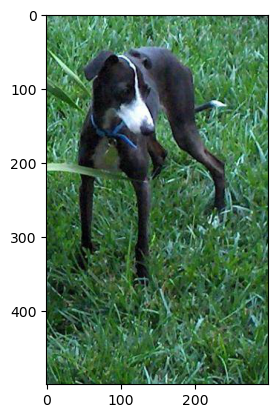
make_predictions('data/presidential_doggy_door/valid/not_bo/121.jpg')
1/1 [==============================] - 0s 156ms/step


array([[36.77488]], dtype=float32)
It looks like a negative number prediction means that it is Bo and a positive number prediction means it is something else. We can use this information to have our doggy door only let Bo in!
Exercise: Bo’s Doggy Door
Fill in the following code to implement Bo’s doggy door:
def presidential_doggy_door(image_path):
    preds = make_predictions(image_path)
    if preds[0] < 0:
        print("It's Bo! Let him in!")
    else:
        print("That's not Bo! Stay out!")
Let’s try it out!
presidential_doggy_door('data/presidential_doggy_door/valid/not_bo/131.jpg')
1/1 [==============================] - 0s 132ms/step
That's not Bo! Stay out!
presidential_doggy_door('data/presidential_doggy_door/valid/bo/bo_29.jpg')
1/1 [==============================] - 0s 110ms/step
It's Bo! Let him in!
Summary
Great work! With transfer learning, you have built a highly accurate model using a very small dataset. This can be an extremely powerful technique, and be the difference between a successful project and one that cannot get off the ground. We hope these techniques can help you out in similar situations in the future!
There is a wealth of helpful resources for transfer learning in the NVIDIA TAO Toolkit.
Clear the Memory
Before moving on, please execute the following cell to clear up the GPU memory.
import IPython
app = IPython.Application.instance()
app.kernel.do_shutdown(True)
Key Points
FIX