Keras & Tensorflow - The MNIST dataset

Overview

Teaching: 30 min
Exercises: 0 min

Questions

• Building a first Deep Learning model to recognize handwritten digits.

Objectives

• FIX

Deep Learning is a subset of Machine Learning that is inspired by the brain’s architecture to build an intelligent machine through the use of artificial neural networks (ANNs) which are the very core of Deep Learning. They are versatile, powerful, and scalable, making them ideal to tackle large and highly complex Machine Learning tasks, such as classifying billions of images and running speech recognition services.

As other Machine Learning algorithms, ANNs have their own set of parameters that need to be specified and tweak in order to create, train and use a model. We will try to exemplify these parameters and steps through solving a very simple deep learning problem. For this we will use Keras API which is a beautifully designed and simple high-level API for building, training, evaluating and running neural networks. Despite its simplicity it is flexible enough to allow you to build a wide variety of neural network architectures.

The MNIST dataset.

We will use the MNIST dataset, a classic machine learning algorithm. The dataset consists of 60,000 training images and 10,000 testing images. Each element in the dataset correspond to a grayscale image of handwritten digits (28x28 pixels). You can think of solving MNIST, this is, classifying each number into one of 10 categories or class, as the “Hello World” of deep learning and can be used to verify that algorithms work correctly.

We can use Keras to work with MNIST since it comes preloaded as a set of four Numpy arrays:

from keras.datasets import mnist
(train_images, train_labels),(test_images, test_labels) = mnist.load_data()

If this is the first time importing mnist, Keras with try to download it from the internet.

Using TensorFlow backend.
Downloading data from https://s3.amazonaws.com/img-datasets/mnist.npz
11493376/11490434 [==============================] - 7s 1us/step

Downloading data in HPC systems

When working on HPC systems is not uncommon that compute or work nodes are close to the outside world for security reasons. In those cases, it is better to try to download any required data locally in the login or head nodes and then instruct your code how to access it.

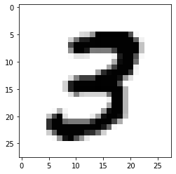
The model will learn from the training set composed by train_images and train_labels and then will be tested on the test set test_images and test_labels. The images are encoded as Numpy arrays, and the labels are an array of digits, ranging from 0 to 9. We can check which digit is placed in position 8 in the training set (remember that numpy arrays are zero-based indexed) with:

print("Digit at position 8:",train_labels[7])

3

If we wanted to see the corresponding image we could use Python’s Matplotlib:

import matplotlib.pyplot as plt
plt.imshow(train_images[7],cmap=plt.cm.binary)

We can further confirm the size of our sets:

print("Number of train images: ", train_images.shape)
print("Number of train labels: ", train_labels.shape)
print("Number of test images: ", test_images.shape)
print("Number of test labels: ", test_labels.shape)

Number of train images:  (60000, 28, 28)
Number of train labels:  (60000,)
Number of test images:  (10000, 28, 28)
Number of test labels:  (10000,)

Building the model

In deep learning algorithms we rely on ANNs which building blocks are the layer, a data processing module that works as a filter for data. Layers are in charge of extracting representations out of the data fed into them. The deep in deep learning comes from chaining together simple layers on top of each other in a kind of data distillation process.

In Keras, Models groups layers into an object with training and inference features. There are three ways to create Keras models: the sequential model, which is simply a list of layers and is limited to single input and single output layers; the functional API, which supports arbitrary model architecture and is applicable to most use cases; and a model subclassing that allows the user to everything from scratch for maximum flexibility. For this course we will use a simple sequential model. We start by importing the necessary libraries and instantiating a model.

from tensorflow.keras import models

network = models.Sequential()

A deep learning model consist of a series of stacked layers. A layer consists of a tensor-in tensor-out computation function. For this example we use two densely connected NN layers. The first one receives a layer of 28 by 28 input elements that corresponds to our images. activation is an element-wise activation function, kernel and bias are a weights matrix and a bias vector created by the layer. The first argument passed to the dense layer indicates the number of nodes in the layer, (or dimensionality of the layer’s output space).

from tensorflow.keras import layers

network.add(layers.Dense(512,activation='relu',input_shape=(28 * 28,)))
network.add(layers.Dense(10,activation='softmax'))

Dense layers implements the operation:

output = activation(dot(input, kernel) + bias)

As mentioned above, activation is a element wise function, there are several types but for this example we use two of the most common ones: relu function, that applies the rectified linear unit activation function; and the softmax function, that converts a real vector to a vector of categorical probabilities. The latter is often used as the activation for the last layer of a classification network because the result could be interpreted as a probability distribution. In this case each score will be the probability that the current digit image belongs to one out of 10 digit classes.

We can find out more details about our network with:

network.summary()

Model: "sequential_3"
_________________________________________________________________
Layer (type)                 Output Shape              Param #   
=================================================================
dense_6 (Dense)              (None, 512)               401920    
_________________________________________________________________
dense_7 (Dense)              (None, 10)                5130      
=================================================================
Total params: 407,050
Trainable params: 407,050
Non-trainable params: 0
_________________________________________________________________
_.

Where a trainable parameter is a parameter that is learned by a network during training. These commonly are the weights and biases of the network but can refer to any other parameter that is learned during training. We can find out how many trainable parameters are in our network by counting the number of parameters within each layer and then sum them up to get the total in the network. For this we need the number of inputs to the layer, its number of outputs (equal to the number of nodes in the layer) and whether or not the layer contains biases (also equal to the number of nodes in the layer). Then we simply multiply the number of inputs and outputs and add the number biases and then add the results for all layers. These parameters are where knowledge of the network persists. If you are curious, you can take a look with:

network.get_weights()

Training

Before actually training our model, there are three parameters that need to be defined as part of a compilation step:

• Loss function: is the function that the network is required to minimize (cost or error function) or maximize (objective function).
• Optimizer: defines how the network should change its weights or learning rates to reduce the losses.
• Metrics: A list of metrics to be evaluated by the model during training and testing. ‘accuracy’ is a typically used metric in Keras models.

network.compile(optimizer='rmsprop',
                loss='categorical_crossentropy',
                metrics=['accuracy'])

The next step is to prepare our data to be fed to the model. As we are expecting the model to output the probability (between 0 and 1) that a digit belongs to 1 of 10 classes, we need to transform our data accordingly.

train_images = train_images.reshape((60000,28 * 28))
train_images = train_images.astype('float32')/255
test_images = test_images.reshape((10000,28 * 28))
test_images = test_images.astype('float32')/255

And we convert the label vectors to binary matrices for use with the categorical crossentropy loss function:

from tensorflow.keras.utils import to_categorical
train_labels = to_categorical(train_labels)
test_labels = to_categorical(test_labels)

We are finally ready to train our model by calling its fit method:

network.fit(train_images,train_labels,epochs=5,batch_size=128)

Epoch 1/5
469/469 [==============================] - 8s 16ms/step - loss: 0.2574 - accuracy: 0.9251
Epoch 2/5
469/469 [==============================] - 4s 9ms/step - loss: 0.1032 - accuracy: 0.9699
Epoch 3/5
469/469 [==============================] - 4s 9ms/step - loss: 0.0678 - accuracy: 0.9797
Epoch 4/5
469/469 [==============================] - 4s 9ms/step - loss: 0.0490 - accuracy: 0.9852
Epoch 5/5
469/469 [==============================] - 4s 9ms/step - loss: 0.0367 - accuracy: 0.9890

Notice that the model’s accuracy increases while the loss value decreases at the end of each epoch. This is the expected behaviour when training a deep learning model. The rate at which learning will occur depends on many parameters and you should try to test alternative algorithms and parameters.

Batches and Epochs

Deep learning models very often don’t process an entire dataset at once (especially when the amount of data is very large), but instead break the data into subsets called batches. For example, one batch of 256 images would simply be:

batch = train_images[:256]

An entire iteration over all the training data is known as an epoch.

Validation

As we did with in our previous machine learning models, it is very useful to measure the degree of confidence we should have in our model by comparing its predictions on data for which we know the real values. For this we use our test dataset:

test_loss, test_acc = network.evaluate(test_images,test_labels)
print('test_acc:',test_acc)

313/313 [==============================] - 1s 3ms/step - loss: 0.0654 - accuracy: 0.9801
test_acc: 0.9800999760627747

Our model reached an accuracy of 0.98% for the validation data set which is slightly lower than the accuracy obtained with the training data, which is an example of overfitting.

Hopefully solving this very simple deep learning exercise will allow your quest to tackle more complex problems in your work.

Key Points

• FIX