Scikit Learn - The Iris Dataset

Overview

Teaching: 60 min
Exercises: 0 min

Questions

• Use Scikit Learn to build a simple classification Machine Learning model.

Objectives

• Understand the use of the k-neareast neighbours algorithm.

• Familizarize with using subsets of the features available in our training set.

• Plot decision boundaries in classification algorithms.

In this lesson we will use a popular machine learning example, the Iris dataset, to understand some of the most basic concepts around machine learning applications. For this, we will employ Scikit-learn one of the most popular and prominent Python library for machine learning. Scikit-learn comes with a few standard datasets, for instance the iris and digits datasets for classification and the diabetes dataset for regression, you can find more information about these and other datasets in the context of Scikit-learn usage here.

The Iris Dataset

The data set consists of 50 samples from each of three species of Iris (Iris setosa, Iris virginica and Iris versicolor). Four features were measured from each sample: the length and the width of the sepals and petals, in centimeters. You can find out more about this dataset here and here.

Features

In machine learning datasets, each entity or row here is known as a sample (or data point), while the columns—the properties that describe these entities—are called features.

To start our work we can open a new Python session and import our dataset:

from sklearn.datasets import load_iris
iris_dataset = load_iris()

Datasets

In general, in machine learning applications, a dataset is a dictionary-like object that holds all the data and some metadata about the data. In particular, when we use Scikit-learn data loaders we obtain an object of type Bunch:

type(iris_dataset)

sklearn.utils.Bunch

This type of object is a container that exposes its keys as attributes. You can find out more about Scikit-learn Bunch objects here.

Take a look at the keys in our newly loaded dataset:

print("Keys of iris_dataset: \n{}".format(iris_dataset.keys()))

Keys of iris_dataset: 
dict_keys(['data', 'target', 'frame', 'target_names', 'DESCR', 'feature_names', 'filename'])

The dataset consists of the following sections:

• data: contains the numeric measurements of sepal length, sepal width, petal length, and petal width in a NumPy array. The array contains 4 measurements (features) for 150 different flowers (samples).
• target: contains the species of each of the flowers that were measured, also as a NumPy array. Each entry consists of a integer number in the set 0, 1 or 2.
• target_names: contains the meanings of the numbers given in the target_names array: 0 means setosa, 1 means versicolor, and 2 means virginica.
• DESCR: a short description of the dataset.
• feature_names: a list of strings, giving the description of each feature in data.
• filename: location where the dataset is stored.

And we can explore the contents of these sections:

print("First five columns of data:\n{}".format(iris_dataset['data'][:5]))
print("\n")
print("Targets:\n{}".format(iris_dataset['target'][:]))
print("\n")
print("Target names:\n{}".format(iris_dataset['target_names']))
print("\n")
print("Feature names:\n{}".format(iris_dataset['feature_names']))
print("\n")
print("Dataset location:\n{}".format(iris_dataset['filename']))

First five columns of data:
[[5.1 3.5 1.4 0.2]
 [4.9 3.  1.4 0.2]
 [4.7 3.2 1.3 0.2]
 [4.6 3.1 1.5 0.2]
 [5.  3.6 1.4 0.2]]


Targets:
[0 0 0 0 0 0 0 0 0 0 0 0 0 0 0 0 0 0 0 0 0 0 0 0 0 0 0 0 0 0 0 0 0 0 0 0 0
 0 0 0 0 0 0 0 0 0 0 0 0 0 1 1 1 1 1 1 1 1 1 1 1 1 1 1 1 1 1 1 1 1 1 1 1 1
 1 1 1 1 1 1 1 1 1 1 1 1 1 1 1 1 1 1 1 1 1 1 1 1 1 1 2 2 2 2 2 2 2 2 2 2 2
 2 2 2 2 2 2 2 2 2 2 2 2 2 2 2 2 2 2 2 2 2 2 2 2 2 2 2 2 2 2 2 2 2 2 2 2 2
 2 2]


Target names:
['setosa' 'versicolor' 'virginica']


Feature names:
['sepal length (cm)', 'sepal width (cm)', 'petal length (cm)', 'petal width (cm)']


Dataset location:
/home/vagrant/anaconda3/envs/deep-learning/lib/python3.7/site-packages/sklearn/datasets/data/iris.csv

In particular, try printing the content of the DESCR key:

print(iris_dataset['DESCR'])

.. iris_dataset:

Iris plants dataset
--------------------

**Data Set Characteristics:**

    :Number of Instances: 150 (50 in each of three classes)
    :Number of Attributes: 4 numeric, predictive attributes and the class
    :Attribute Information:
        - sepal length in cm
        - sepal width in cm
        - petal length in cm
        - petal width in cm
        - class:
                - Iris-Setosa
                - Iris-Versicolour
                - Iris-Virginica
                
    :Summary Statistics:

    ============== ==== ==== ======= ===== ====================
                    Min  Max   Mean    SD   Class Correlation
    ============== ==== ==== ======= ===== ====================
    sepal length:   4.3  7.9   5.84   0.83    0.7826
    sepal width:    2.0  4.4   3.05   0.43   -0.4194
    petal length:   1.0  6.9   3.76   1.76    0.9490  (high!)
    petal width:    0.1  2.5   1.20   0.76    0.9565  (high!)
    ============== ==== ==== ======= ===== ====================

    :Missing Attribute Values: None
    :Class Distribution: 33.3% for each of 3 classes.
    :Creator: R.A. Fisher
    :Donor: Michael Marshall (MARSHALL%PLU@io.arc.nasa.gov)
    :Date: July, 1988

The famous Iris database, first used by Sir R.A. Fisher. The dataset is taken
from Fisher's paper. Note that it's the same as in R, but not as in the UCI
Machine Learning Repository, which has two wrong data points.

This is perhaps the best known database to be found in the
pattern recognition literature.  Fisher's paper is a classic in the field and
is referenced frequently to this day.  (See Duda & Hart, for example.)  The
data set contains 3 classes of 50 instances each, where each class refers to a
type of iris plant.  One class is linearly separable from the other 2; the
latter are NOT linearly separable from each other.

.. topic:: References

   - Fisher, R.A. "The use of multiple measurements in taxonomic problems"
     Annual Eugenics, 7, Part II, 179-188 (1936); also in "Contributions to
     Mathematical Statistics" (John Wiley, NY, 1950).
   - Duda, R.O., & Hart, P.E. (1973) Pattern Classification and Scene Analysis.
     (Q327.D83) John Wiley & Sons.  ISBN 0-471-22361-1.  See page 218.
   - Dasarathy, B.V. (1980) "Nosing Around the Neighborhood: A New System
     Structure and Classification Rule for Recognition in Partially Exposed
     Environments".  IEEE Transactions on Pattern Analysis and Machine
     Intelligence, Vol. PAMI-2, No. 1, 67-71.
   - Gates, G.W. (1972) "The Reduced Nearest Neighbor Rule".  IEEE Transactions
     on Information Theory, May 1972, 431-433.
   - See also: 1988 MLC Proceedings, 54-64.  Cheeseman et al"s AUTOCLASS II
     conceptual clustering system finds 3 classes in the data.
   - Many, many more ...

Test vs training sets

To assess the model’s performance, we show it new data (data that it hasn’t seen before) for which we have labels. This is usually done by splitting the labeled data we have collected (here, our 150 flower measurements) into two parts. One part of the data is used to build our machine learning model, and is called the training data or training set. The rest of the data will be used to assess how well the model works; this is called the test data, test set, or hold-out set.

Unfortunately, we cannot use the data we used to build the model to evaluate it. This is because our model could always simply remember the whole training set (overfitting), and will therefore always predict the correct label for any point in the training set. This “remembering” does not indicate to us whether our model will generalize well (in other words, whether it will also perform well on new data).

Training

Scikit-learn’s train_test_split function allow us to shuffle and split the dataset in a single line. The function takes a sequence of arrays (the arrays must be of the same length) and options to specify how to split the arrays. By default, the function extracts 75% of the rows in the arrays as the training set while the remaining 25% of rows is declared as the test set. Deciding how much data you want to put into the training and the test set respectively is somewhat arbitrary, but using a test set containing 25% of the data is a good rule of thumb. The function also allow us to control the shuffling applied to the data before applying the split with the option random_state, this ensures reproducible results.

from sklearn.model_selection import train_test_split

X_train, X_test, y_train, y_test = train_test_split(
        iris_dataset['data'], iris_dataset['target'], test_size=0.25, random_state=0)
print("X_train shape: {}".format(X_train.shape)) 
print("y_train shape: {}".format(y_train.shape))
print("X_test shape: {}".format(X_test.shape)) 
print("y_test shape: {}".format(y_test.shape))

X_train shape: (112, 4)
y_train shape: (112,)
X_test shape: (38, 4)
y_test shape: (38,)

We can use Pandas’ plotting function scatter_matrix that draws a matrix of scatter plots to visualize our data. This function takes a dataframe and plots each variable contained within, against each other. The first step is import Pandas and transfor our Numpy array into a Pandas dataframe:

import pandas as pd
iris_dataframe = pd.DataFrame(X_train, columns=iris_dataset.feature_names)
grr = pd.plotting.scatter_matrix(iris_dataframe, c=y_train, figsize=(15, 15), marker='o',hist_kwds={'bins': 20}, s=60, alpha=.8)

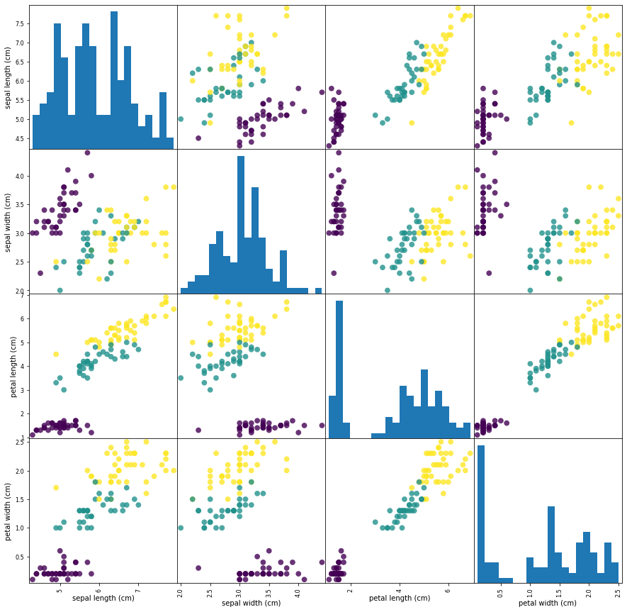
The diagonal in the image shows the distribution of the three numeric variables of our example data. In the other cells of the plot matrix, we have the scatter plots of each variable combination of our dataframe. Take a look at Pandas’ scatter_matrix documentation to find out more about the options we have used. Keep in mind as well that Pandas’ scatter_matrix makes use of Matplotlib’s scatter function under the hood to perform the actual plotting and that we have passed a couple of arguments to this function in our previous command, specifically point color and size options. Find out more at Matplotlib’s scatter function documentation.

Back to the plots, we can see that the three classes seem to be relatively well separated using the sepal and petal measurements. This means that a machine learning model will likely be able to learn to separate them.

Building the model

There are many classification algorithms in scikit-learn that we could use. Here we will use a k-nearest neighbors classifier, which is easy to understand. Neighbors-based classification algorithms are a type of instance-based learning that does not attempt to construct a general internal model, but simply stores instances of the training data. Classification is computed from a simple majority vote of the nearest neighbors of each point: a query point is assigned the data class which has the most representatives within the nearest neighbors of the point.

Building this model only consists of storing the training set. To make a prediction for a new data point, the algorithm finds the point in the training set that is closest to the new point. Then it assigns the label of this training point to the new data point.

from sklearn.neighbors import KNeighborsClassifier
n_neighbors=1
knn = KNeighborsClassifier(n_neighbors=1)

knn becomes an object that contains the algorithm used to build the model using the training dataset as well as to make predictions from new data points. Now we can train our model using the training dataset. We could use all the features of training data set our just a sub set. In this case, to facilitate later visualization, we will only use two features: petal length (cm) and petal width (cm):

knn.fit(X_train[:,2:], y_train)

Plot the decision boundaries

Once again, in order to understand how the model classifies new points, it could be useful to visualize it. For this we can use matplotlib library and plot our training data set on top of a coloured domain in which each color represents a category in our model.

import numpy as np
from matplotlib.colors import ListedColormap
import matplotlib.pyplot as plt

x_min,x_max = X_train[:,2].min() - 1, X_train[:,2].max()+ 1
y_min,y_max = X_train[:,3].min() - 1, X_train[:,3].max()+ 1
h=0.02
xx,yy = np.meshgrid(np.arange(x_min,x_max,h),np.arange(y_min,y_max,h))
Z = knn.predict(np.c_[xx.ravel(), yy.ravel()])
Z = Z.reshape(xx.shape)

cmap_bold = ListedColormap(['darkorange', 'c', 'darkblue'])
cmap_light=ListedColormap(['orange', 'cyan', 'cornflowerblue'])

fig = plt.figure()
ax1 = fig.add_subplot(111)
ax1.pcolormesh(xx, yy, Z, cmap=cmap_light, shading='gouraud')
for target in iris_dataset.target_names:
    index=np.where(iris_dataset.target_names==target)[0][0]
    ax1.scatter(X_train[:,2][y_train==index],X_train[:,3][y_train==index],
                cmap=cmap_bold,edgecolor='k', s=20, label=target)
ax1.set_xlim(x_min,x_max)
ax1.set_ylim(y_min,y_max)
ax1.legend()
ax1.set_xlabel("petal length (cm)")
ax1.set_ylabel("petal width (cm)")
ax1.set_title("3-Class classification (k = %i, weights = '%s')"
              % (n_neighbors, 'uniform'))
plt.show()

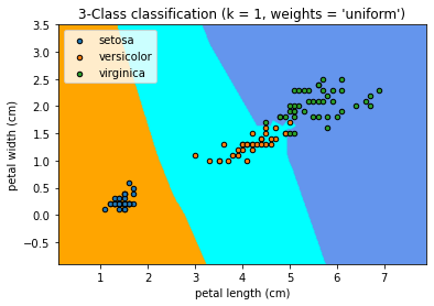
This figure show us the regions where new data points would be classified based on their petal length and width measurements.

Making predictions

With out newly build model, we can now make predictions on new data for which we would like to find the correct labels. Assume you found an iris in the park with a sepal length of 4 cm, a sepal width of 3.5 cm, a petal length of 1.2 cm, and a petal width of 0.5 cm.

new_data=np.array([[4,3.5,1.2,0.5]])
prediction = knn.predict(new_data[:,2:])
print("Prediction: {}".format(prediction))
print("Predicted target name: {}".format(iris_dataset['target_names'][prediction]))

Validate the model

Our model predicts that the iris found in the park belongs to the setosa species. How sure can we be that this is the correct answer? For this, we need to validate our model using the data we set apart for this purpose in which we know the right species for each flower in the set (remember we are working only with 2 features from our data set).

y_pred = knn.predict(X_test[:,2:])
print("Test set predictions:\n {}".format(y_pred))

The above command give us the following output that represents the class for each entry in the validation dataset:

Test set predictions:
 [2 1 0 2 0 2 0 1 1 1 2 1 1 1 1 0 1 1 0 0 2 1 0 0 2 0 0 1 1 0 2 1 0 2 2 1 0 2]

And now we can compare the above predicted classes with their actual values and obtain a measure (accuracy) of how well our model works.

print("Test set score: {:.2f}".format(knn.score(X_test[:,2:], y_test)))

Test set score: 0.97

Now we could say that we are 97% sure that the iris we found at the park belongs to the setosa species. You can try to use a different set of features or maybe all of them and see if you can improve this value (be aware of overfitting your model).

Key Points

• k-Nearest Neighbors is a simple classification algorithm in which predictions a new data point to the closest data points in the training dataset.

• It is not necessary to use all the features in our training dataset. We can use different combinations to try to achive better results.