Testing our environment

Overview

Teaching: 45 min
Exercises: 0 min

Questions

• Use Scikit Learn to build a simple linear regression machine learning problem.

Objectives

• Familiarize with the basic steps involved in building a machine learning model.

• Test our machine learning tools and environment.

GDP and happiness

We will start building a very simple model to predict people Happiness (as measured by the OECD) based on the country’s GDP (as provided by the IMF). This is also called model-based learning. For this course we will use Scikit-Learn but other libraries should provide similar functionalities.

Obtaining and working with data

When developing Machine Learning applications you will likely need to work with databases either by creating them yourself or obtaining some already available. Depending on the field and stage of your research, the databases can range from a few megabytes to several hundreds gigabytes and ever bigger. At that point you’ll likely need to consider carefully (even more if the database has data protection requirements) how best to manage storage requirements in order to optimize available resources in your work system. Do not hesitate to contact your system administrators to discuss further any doubts or concerns that you might have.

Luckily for this training the databases we will be working with are publicly available from the OECD’s Better Life Index) and the IMF’s GDP per capita) and only occupy a few megabytes. You can also find them in the zip file provided for this training course.

Start by loading some python libraries.

import matplotlib.pyplot as plt
import numpy as np
import pandas as pd
import sklearn.linear_model

Continue by loading the data as Pandas dataframes. For this you need to provide the corresponding file locations, for example:

file_gdp="gdp-bli/gdp_per_capita_2014-2025.csv"
file_happy="gdp-bli/BLI_25112020150937807.csv"

df_gdp=pd.read_csv(file_gdp,thousands=',',delimiter='\t',encoding='latin1',na_values='n/a')
df_happy=pd.read_csv(file_happy,thousands=',')

You can take a look at the data we just loaded with the head dataframe function, for example, to print the first 5 rows in the GDP dataframe:

rows=5
df_gdp.head(rows)

Next we define a helper function to filter and restructure OECD’s data in a more suitable way; rename the column corresponding to 2020 in IMF’s GDP per capita data and set the country name as index; we then merge the dataframes using their indexes (country name) and sort the resulting dataframe by GDP value (in ascending order). To emulate the creation of a test dataset we save only a subset of our newly created dataframe. Some of the removed datapoints correspond to South Africa, Colombia, Iceland and Denmark. We can later use the data corresponding to these countries to validate our Machine Learning Model.

def prepare_country_stats(data_happy,data_gdp):
    # Process happiness data
    # select rows matching TOT in columns INEQUALITY
    data_happy = data_happy[data_happy["INEQUALITY"]=="TOT"]
    # Create new df using 'Country' column as index and 'Indicator' as columns
    # df is populated using values from column 'Values'
    data_happy = data_happy.pivot(index="Country", columns="Indicator",values="Value")

    # Process GDP data
    # rename column and set a new index
    data_gdp = data_gdp.rename(columns={"2021":"GDP per capita (2020)"})
    data_gdp = data_gdp.set_index("Country")
    
    # Merge both datasets by country
    merged_data = pd.merge(left=data_happy, right=data_gdp,left_index=True, right_index=True)
    merged_data.sort_values(by="GDP per capita (2020)",inplace=True)
    
    # Create two sub datasets for testing and validation
    # We select two specific columns out of the merged dataset
    remove_indices = [0, 1, 6, 8, 33, 34, 35, 36, 37, 38, 39]
    keep_indices = list(set(range(merged_data.shape[0])) - set(remove_indices))
    
    test_data     = merged_data[["GDP per capita (2020)",'Life satisfaction']].iloc[keep_indices]
    validate_data = merged_data[["GDP per capita (2020)",'Life satisfaction']].iloc[remove_indices]
    
    return test_data, validate_data

Use the previously defined helper function and extract the data for “GDP per capita (2020)” and “Life satisfaction” as column vectors using Numpy.

country_stats_test, country_stats_validate = prepare_country_stats(df_happy,df_gdp)
x = np.c_[country_stats_test["GDP per capita (2020)"]]
y = np.c_[country_stats_test["Life satisfaction"]]

Building the model

At this point it might be useful to visualize our data in order to gain some insight about the type of model that might be more useful to describe it:

country_stats_test.plot(kind='scatter', x="GDP per capita (2020)", y='Life satisfaction',xlim=[0,60000],ylim=[0,10])
plt.show()

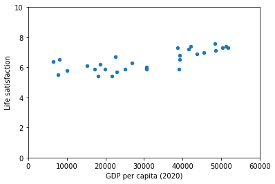
There does seem to be a trend here! Although the data is noisy (i.e., partly random), it looks like life satisfaction goes up more or less linearly as the country’s GDP per capita increases. So you decide to model life satisfaction as a linear function of GDP per capita. This step is called model selection: you selected a linear model of life satisfaction with just one attribute, GDP per capita:

model = sklearn.linear_model.LinearRegression()

With the model selected, the next step is to fit it to the data. The calculations performed in this step are model dependent, for example, for a linear model it involves calculating a set of coefficients to minimize the residual sum of squares between the observed targets in the dataset, and the targets predicted by the linear approximation.

model.fit(x, y)

And we can access the estimated value for the model key parameters (which parameters are available also depends on the selected model).

print(f"model's intercept: {model.intercept_[0]}")
print(f"model's slope    : {model.coef_[0][0]}")

model's intercept: 5.375355125502892
model's slope    : 3.563396686332422e-05

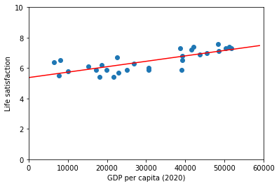
It might be useful to plot our model along side our data:

fig = plt.figure()
ax1 = fig.add_subplot(111)
ax1.scatter(country_stats_test["GDP per capita (2020)"],country_stats_test["Life satisfaction"])
ax1.set_xlim(0,60000)
ax1.set_ylim(0,10)
ax1.set_xlabel("GDP per capita (2020)")
ax1.set_ylabel("Life satisfaction")
x_val=np.array([list(range(0,60000,1000))]).T
ax1.plot(x_val, model.predict(x_val),color='r')
plt.show()

Validating and making predictions

After we have trained our model we should perform some validation checks using the labelled data we saved for this purpose:

print("Country               GDP  BLI(pred) BLI")
for country, row in country_stats_validate.iterrows():
    gdp_real = row[0]
    bli_real = row[1]
    gdp_pred = model.predict([[gdp_real]])
    print("{0:14}  {1:9.2f}  {2:5.2f}  {3:7.2f}".format(country, gdp_real, gdp_pred[0][0], bli_real))

Country               GDP  BLI(pred) BLI
South Africa      4735.75   5.54     4.70
Colombia          5207.24   5.56     6.30
Chile            12612.32   5.82     6.50
Hungary          15372.89   5.92     5.60
Iceland          57189.03   7.41     7.50
Denmark          58438.85   7.46     7.60
United States    63051.40   7.62     6.90
Norway           67988.59   7.80     7.60
Ireland          79668.50   8.21     7.00
Switzerland      81867.46   8.29     7.50
Luxembourg      109602.32   9.28     6.90

Always helpful to have some visual aids to compare how well our model does compared with the validation data

fig = plt.figure()
ax1 = fig.add_subplot(111)
ax1.scatter(country_stats_test["GDP per capita (2020)"],country_stats_test["Life satisfaction"])
ax1.set_xlim(0,110000)
ax1.set_ylim(0,10)
ax1.set_xlabel("GDP per capita (2020)")
ax1.set_ylabel("Life satisfaction")
x_val=np.array([list(range(0,60000,1000))]).T
ax1.plot(x_val, model.predict(x_val),color='r')
ax1.scatter(country_stats_validate["GDP per capita (2020)"],country_stats_validate["Life satisfaction"],color='g')
plt.show()

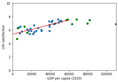
Seems like our model is reasonably good at predicting values that fall within the range of our training data set but tends to overestimate the observed life satisfaction of richer countries. This give us an idea of the degree of confidence that we should have in our very simple model, perhaps we should try modifying the model parameters or adding other variables like employment rate, health, air pollution and employ slighly more complex models.

Key Points

• Python is a very useful programming language to develop machine learning applications

• Scikit Learn together with Numpy, Pandas and Matplotlib form a popular machine learning environment.

• Linear regression is one of the most simple and useful machine learning algorithms in which the model makes a prediction by simply computing a weighted sum of the input features, plus a constant called the intercept term.