Python Fundamentals

Overview

Teaching: 20 min
Exercises: 10 min

Questions

• What basic data types can I work with in Python?

• How can I create a new variable in Python?

• How do I use a function?

• Can I change the value associated with a variable after I create it?

Objectives

• Assign values to variables.

Variables

Any Python interpreter can be used as a calculator:

3 + 5 * 4

23

This is great but not very interesting. To do anything useful with data, we need to assign its value to a variable. In Python, we can assign a value to a variable, using the equals sign =. For example, we can track the weight of a patient who weighs 60 kilograms by assigning the value 60 to a variable weight_kg:

weight_kg = 60

From now on, whenever we use weight_kg, Python will substitute the value we assigned to it. In layman’s terms, a variable is a name for a value.

In Python, variable names:

• can include letters, digits, and underscores
• cannot start with a digit
• are case sensitive.

This means that, for example:

• weight0 is a valid variable name, whereas 0weight is not
• weight and Weight are different variables

Types of data

Python knows various types of data. Three common ones are:

• integer numbers
• floating point numbers, and
• strings.

In the example above, variable weight_kg has an integer value of 60. If we want to more precisely track the weight of our patient, we can use a floating point value by executing:

weight_kg = 60.3

To create a string, we add single or double quotes around some text. To identify and track a patient throughout our study, we can assign each person a unique identifier by storing it in a string:

patient_id = '001'

Using Variables in Python

Once we have data stored with variable names, we can make use of it in calculations. We may want to store our patient’s weight in pounds as well as kilograms:

weight_lb = 2.2 * weight_kg

We might decide to add a prefix to our patient identifier:

patient_id = 'inflam_' + patient_id

Built-in Python functions

To carry out common tasks with data and variables in Python, the language provides us with several built-in functions. To display information to the screen, we use the print function:

print(weight_lb)
print(patient_id)

132.66
inflam_001

When we want to make use of a function, referred to as calling the function, we follow its name by parentheses. The parentheses are important: if you leave them off, the function doesn’t actually run! Sometimes you will include values or variables inside the parentheses for the function to use. In the case of print, we use the parentheses to tell the function what value we want to display. We will learn more about how functions work and how to create our own in later episodes.

We can display multiple things at once using only one print call:

print(patient_id, 'weight in kilograms:', weight_kg)

inflam_001 weight in kilograms: 60.3

We can also call a function inside of another function call. For example, Python has a built-in function called type that tells you a value’s data type:

print(type(60.3))
print(type(patient_id))

<class 'float'>
<class 'str'>

Moreover, we can do arithmetic with variables right inside the print function:

print('weight in pounds:', 2.2 * weight_kg)

weight in pounds: 132.66

The above command, however, did not change the value of weight_kg:

print(weight_kg)

60.3

To change the value of the weight_kg variable, we have to assign weight_kg a new value using the equals = sign:

weight_kg = 65.0
print('weight in kilograms is now:', weight_kg)

weight in kilograms is now: 65.0

Variables as Sticky Notes

A variable in Python is analogous to a sticky note with a name written on it: assigning a value to a variable is like putting that sticky note on a particular value.

Using this analogy, we can investigate how assigning a value to one variable does not change values of other, seemingly related, variables. For example, let’s store the subject’s weight in pounds in its own variable:

# There are 2.2 pounds per kilogram
weight_lb = 2.2 * weight_kg
print('weight in kilograms:', weight_kg, 'and in pounds:', weight_lb)

weight in kilograms: 65.0 and in pounds: 143.0

Similar to above, the expression 2.2 * weight_kg is evaluated to 143.0, and then this value is assigned to the variable weight_lb (i.e. the sticky note weight_lb is placed on 143.0). At this point, each variable is “stuck” to completely distinct and unrelated values.

Let’s now change weight_kg:

weight_kg = 100.0
print('weight in kilograms is now:', weight_kg, 'and weight in pounds is still:', weight_lb)

weight in kilograms is now: 100.0 and weight in pounds is still: 143.0

Since weight_lb doesn’t “remember” where its value comes from, it is not updated when we change weight_kg.

Check Your Understanding

What values do the variables mass and age have after each of the following statements? Test your answer by executing the lines.

mass = 47.5
age = 122
mass = mass * 2.0
age = age - 20

Solution

`mass` holds a value of 47.5, `age` does not exist
`mass` still holds a value of 47.5, `age` holds a value of 122
`mass` now has a value of 95.0, `age`'s value is still 122
`mass` still has a value of 95.0, `age` now holds 102

Sorting Out References

Python allows you to assign multiple values to multiple variables in one line by separating the variables and values with commas. What does the following program print out?

first, second = 'Grace', 'Hopper'
third, fourth = second, first
print(third, fourth)

Solution

Hopper Grace

Seeing Data Types

What are the data types of the following variables?

planet = 'Earth'
apples = 5
distance = 10.5

Solution

print(type(planet))
print(type(apples))
print(type(distance))

<class 'str'>
<class 'int'>
<class 'float'>

Key Points

• Basic data types in Python include integers, strings, and floating-point numbers.

• Use variable = value to assign a value to a variable in order to record it in memory.

• Variables are created on demand whenever a value is assigned to them.

• Use print(something) to display the value of something.

• Built-in functions are always available to use.

Analyzing Patient Data

Overview

Teaching: 45 min
Exercises: 20 min

Questions

• How can I process tabular data files in Python?

Objectives

• Explain what a library is and what libraries are used for.

• Import a Python library and use the functions it contains.

• Read tabular data from a file into a program.

• Select individual values and subsections from data.

• Perform operations on arrays of data.

Words are useful, but what’s more useful are the sentences and stories we build with them. Similarly, while a lot of powerful, general tools are built into Python, specialized tools built up from these basic units live in libraries that can be called upon when needed.

Loading data into Python

To begin processing inflammation data, we need to load it into Python. We can do that using a library called NumPy, which stands for Numerical Python. In general, you should use this library when you want to do fancy things with lots of numbers, especially if you have matrices or arrays. To tell Python that we’d like to start using NumPy, we need to import it:

import numpy

Importing a library is like getting a piece of lab equipment out of a storage locker and setting it up on the bench. Libraries provide additional functionality to the basic Python package, much like a new piece of equipment adds functionality to a lab space. Just like in the lab, importing too many libraries can sometimes complicate and slow down your programs - so we only import what we need for each program.

Once we’ve imported the library, we can ask the library to read our data file for us:

numpy.loadtxt(fname='inflammation-01.csv', delimiter=',')

array([[ 0.,  0.,  1., ...,  3.,  0.,  0.],
       [ 0.,  1.,  2., ...,  1.,  0.,  1.],
       [ 0.,  1.,  1., ...,  2.,  1.,  1.],
       ...,
       [ 0.,  1.,  1., ...,  1.,  1.,  1.],
       [ 0.,  0.,  0., ...,  0.,  2.,  0.],
       [ 0.,  0.,  1., ...,  1.,  1.,  0.]])

The expression numpy.loadtxt(...) is a function call that asks Python to run the function loadtxt which belongs to the numpy library. This dotted notation is used everywhere in Python: the thing that appears before the dot contains the thing that appears after.

As an example, John Smith is the John that belongs to the Smith family. We could use the dot notation to write his name smith.john, just as loadtxt is a function that belongs to the numpy library.

numpy.loadtxt has two parameters: the name of the file we want to read and the delimiter that separates values on a line. These both need to be character strings (or strings for short), so we put them in quotes.

Since we haven’t told it to do anything else with the function’s output, the notebook displays it. In this case, that output is the data we just loaded. By default, only a few rows and columns are shown (with ... to omit elements when displaying big arrays). Note that, to save space when displaying NumPy arrays, Python does not show us trailing zeros, so 1.0 becomes 1..

Our call to numpy.loadtxt read our file but didn’t save the data in memory. To do that, we need to assign the array to a variable. In a similar manner to how we assign a single value to a variable, we can also assign an array of values to a variable using the same syntax. Let’s re-run numpy.loadtxt and save the returned data:

data = numpy.loadtxt(fname='inflammation-01.csv', delimiter=',')

This statement doesn’t produce any output because we’ve assigned the output to the variable data. If we want to check that the data have been loaded, we can print the variable’s value:

print(data)

[[ 0.  0.  1. ...,  3.  0.  0.]
 [ 0.  1.  2. ...,  1.  0.  1.]
 [ 0.  1.  1. ...,  2.  1.  1.]
 ...,
 [ 0.  1.  1. ...,  1.  1.  1.]
 [ 0.  0.  0. ...,  0.  2.  0.]
 [ 0.  0.  1. ...,  1.  1.  0.]]

Now that the data are in memory, we can manipulate them. First, let’s ask what type of thing data refers to:

print(type(data))

<class 'numpy.ndarray'>

The output tells us that data currently refers to an N-dimensional array, the functionality for which is provided by the NumPy library. These data correspond to arthritis patients’ inflammation. The rows are the individual patients, and the columns are their daily inflammation measurements.

Data Type

A Numpy array contains one or more elements of the same type. The type function will only tell you that a variable is a NumPy array but won’t tell you the type of thing inside the array. We can find out the type of the data contained in the NumPy array.

print(data.dtype)

float64

This tells us that the NumPy array’s elements are floating-point numbers.

With the following command, we can see the array’s shape:

print(data.shape)

(60, 40)

The output tells us that the data array variable contains 60 rows and 40 columns. When we created the variable data to store our arthritis data, we did not only create the array; we also created information about the array, called members or attributes. This extra information describes data in the same way an adjective describes a noun. data.shape is an attribute of data which describes the dimensions of data. We use the same dotted notation for the attributes of variables that we use for the functions in libraries because they have the same part-and-whole relationship.

If we want to get a single number from the array, we must provide an index in square brackets after the variable name, just as we do in math when referring to an element of a matrix. Our inflammation data has two dimensions, so we will need to use two indices to refer to one specific value:

print('first value in data:', data[0, 0])

first value in data: 0.0

print('middle value in data:', data[30, 20])

middle value in data: 13.0

The expression data[30, 20] accesses the element at row 30, column 20. While this expression may not surprise you, data[0, 0] might. Programming languages like Fortran, MATLAB and R start counting at 1 because that’s what human beings have done for thousands of years. Languages in the C family (including C++, Java, Perl, and Python) count from 0 because it represents an offset from the first value in the array (the second value is offset by one index from the first value). This is closer to the way that computers represent arrays (if you are interested in the historical reasons behind counting indices from zero, you can read Mike Hoye’s blog post). As a result, if we have an M×N array in Python, its indices go from 0 to M-1 on the first axis and 0 to N-1 on the second. It takes a bit of getting used to, but one way to remember the rule is that the index is how many steps we have to take from the start to get the item we want.

In the Corner

What may also surprise you is that when Python displays an array, it shows the element with index [0, 0] in the upper left corner rather than the lower left. This is consistent with the way mathematicians draw matrices but different from the Cartesian coordinates. The indices are (row, column) instead of (column, row) for the same reason, which can be confusing when plotting data.

Slicing data

An index like [30, 20] selects a single element of an array, but we can select whole sections as well. For example, we can select the first ten days (columns) of values for the first four patients (rows) like this:

print(data[0:4, 0:10])

[[ 0.  0.  1.  3.  1.  2.  4.  7.  8.  3.]
 [ 0.  1.  2.  1.  2.  1.  3.  2.  2.  6.]
 [ 0.  1.  1.  3.  3.  2.  6.  2.  5.  9.]
 [ 0.  0.  2.  0.  4.  2.  2.  1.  6.  7.]]

The slice 0:4 means, “Start at index 0 and go up to, but not including, index 4”. Again, the up-to-but-not-including takes a bit of getting used to, but the rule is that the difference between the upper and lower bounds is the number of values in the slice.

We don’t have to start slices at 0:

print(data[5:10, 0:10])

[[ 0.  0.  1.  2.  2.  4.  2.  1.  6.  4.]
 [ 0.  0.  2.  2.  4.  2.  2.  5.  5.  8.]
 [ 0.  0.  1.  2.  3.  1.  2.  3.  5.  3.]
 [ 0.  0.  0.  3.  1.  5.  6.  5.  5.  8.]
 [ 0.  1.  1.  2.  1.  3.  5.  3.  5.  8.]]

We also don’t have to include the upper and lower bound on the slice. If we don’t include the lower bound, Python uses 0 by default; if we don’t include the upper, the slice runs to the end of the axis, and if we don’t include either (i.e., if we use ‘:’ on its own), the slice includes everything:

small = data[:3, 36:]
print('small is:')
print(small)

The above example selects rows 0 through 2 and columns 36 through to the end of the array.

small is:
[[ 2.  3.  0.  0.]
 [ 1.  1.  0.  1.]
 [ 2.  2.  1.  1.]]

Analyzing data

NumPy has several useful functions that take an array as input to perform operations on its values. If we want to find the average inflammation for all patients on all days, for example, we can ask NumPy to compute data’s mean value:

print(numpy.mean(data))

6.14875

mean is a function that takes an array as an argument.

Not All Functions Have Input

Generally, a function uses inputs to produce outputs. However, some functions produce outputs without needing any input. For example, checking the current time doesn’t require any input.

import time
print(time.ctime())

Sat Mar 26 13:07:33 2016

For functions that don’t take in any arguments, we still need parentheses (()) to tell Python to go and do something for us.

Let’s use three other NumPy functions to get some descriptive values about the dataset. We’ll also use multiple assignment, a convenient Python feature that will enable us to do this all in one line.

maxval, minval, stdval = numpy.max(data), numpy.min(data), numpy.std(data)

print('maximum inflammation:', maxval)
print('minimum inflammation:', minval)
print('standard deviation:', stdval)

Here we’ve assigned the return value from numpy.max(data) to the variable maxval, the value from numpy.min(data) to minval, and so on.

maximum inflammation: 20.0
minimum inflammation: 0.0
standard deviation: 4.61383319712

Mystery Functions in IPython

How did we know what functions NumPy has and how to use them? If you are working in IPython or in a Jupyter Notebook, there is an easy way to find out. If you type the name of something followed by a dot, then you can use tab completion (e.g. type numpy. and then press Tab) to see a list of all functions and attributes that you can use. After selecting one, you can also add a question mark (e.g. numpy.cumprod?), and IPython will return an explanation of the method! This is the same as doing help(numpy.cumprod). Similarly, if you are using the “plain vanilla” Python interpreter, you can type numpy. and press the Tab key twice for a listing of what is available. You can then use the help() function to see an explanation of the function you’re interested in, for example: help(numpy.cumprod).

When analyzing data, though, we often want to look at variations in statistical values, such as the maximum inflammation per patient or the average inflammation per day. One way to do this is to create a new temporary array of the data we want, then ask it to do the calculation:

patient_0 = data[0, :] # 0 on the first axis (rows), everything on the second (columns)
print('maximum inflammation for patient 0:', numpy.max(patient_0))

maximum inflammation for patient 0: 18.0

Everything in a line of code following the ‘#’ symbol is a comment that is ignored by Python. Comments allow programmers to leave explanatory notes for other programmers or their future selves.

We don’t actually need to store the row in a variable of its own. Instead, we can combine the selection and the function call:

print('maximum inflammation for patient 2:', numpy.max(data[2, :]))

maximum inflammation for patient 2: 19.0

What if we need the maximum inflammation for each patient over all days (as in the next diagram on the left) or the average for each day (as in the diagram on the right)? As the diagram below shows, we want to perform the operation across an axis:

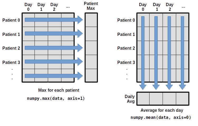
To support this functionality, most array functions allow us to specify the axis we want to work on. If we ask for the average across axis 0 (rows in our 2D example), we get:

print(numpy.mean(data, axis=0))

[  0.           0.45         1.11666667   1.75         2.43333333   3.15
   3.8          3.88333333   5.23333333   5.51666667   5.95         5.9
   8.35         7.73333333   8.36666667   9.5          9.58333333
  10.63333333  11.56666667  12.35        13.25        11.96666667
  11.03333333  10.16666667  10.           8.66666667   9.15         7.25
   7.33333333   6.58333333   6.06666667   5.95         5.11666667   3.6
   3.3          3.56666667   2.48333333   1.5          1.13333333
   0.56666667]

As a quick check, we can ask this array what its shape is:

print(numpy.mean(data, axis=0).shape)

(40,)

The expression (40,) tells us we have an N×1 vector, so this is the average inflammation per day for all patients. If we average across axis 1 (columns in our 2D example), we get:

print(numpy.mean(data, axis=1))

[ 5.45   5.425  6.1    5.9    5.55   6.225  5.975  6.65   6.625  6.525
  6.775  5.8    6.225  5.75   5.225  6.3    6.55   5.7    5.85   6.55
  5.775  5.825  6.175  6.1    5.8    6.425  6.05   6.025  6.175  6.55
  6.175  6.35   6.725  6.125  7.075  5.725  5.925  6.15   6.075  5.75
  5.975  5.725  6.3    5.9    6.75   5.925  7.225  6.15   5.95   6.275  5.7
  6.1    6.825  5.975  6.725  5.7    6.25   6.4    7.05   5.9  ]

which is the average inflammation per patient across all days.

Slicing Strings

A section of an array is called a slice. We can take slices of character strings as well:

element = 'oxygen'
print('first three characters:', element[0:3])
print('last three characters:', element[3:6])

first three characters: oxy
last three characters: gen

What is the value of element[:4]? What about element[4:]? Or element[:]?

Solution

oxyg
en
oxygen

What is element[-1]? What is element[-2]?

Solution

n
e

Given those answers, explain what element[1:-1] does.

Solution

Creates a substring from index 1 up to (not including) the final index, effectively removing the first and last letters from ‘oxygen’

How can we rewrite the slice for getting the last three characters of element, so that it works even if we assign a different string to element? Test your solution with the following strings: carpentry, clone, hi.

Solution

element = 'oxygen'
print('last three characters:', element[-3:])
element = 'carpentry'
print('last three characters:', element[-3:])
element = 'clone'
print('last three characters:', element[-3:])
element = 'hi'
print('last three characters:', element[-3:])

last three characters: gen
last three characters: try
last three characters: one
last three characters: hi

Thin Slices

The expression element[3:3] produces an empty string, i.e., a string that contains no characters. If data holds our array of patient data, what does data[3:3, 4:4] produce? What about data[3:3, :]?

Solution

array([], shape=(0, 0), dtype=float64)
array([], shape=(0, 40), dtype=float64)

Stacking Arrays

Arrays can be concatenated and stacked on top of one another, using NumPy’s vstack and hstack functions for vertical and horizontal stacking, respectively.

import numpy

A = numpy.array([[1,2,3], [4,5,6], [7, 8, 9]])
print('A = ')
print(A)

B = numpy.hstack([A, A])
print('B = ')
print(B)

C = numpy.vstack([A, A])
print('C = ')
print(C)

A =
[[1 2 3]
 [4 5 6]
 [7 8 9]]
B =
[[1 2 3 1 2 3]
 [4 5 6 4 5 6]
 [7 8 9 7 8 9]]
C =
[[1 2 3]
 [4 5 6]
 [7 8 9]
 [1 2 3]
 [4 5 6]
 [7 8 9]]

Write some additional code that slices the first and last columns of A, and stacks them into a 3x2 array. Make sure to print the results to verify your solution.

Solution

A ‘gotcha’ with array indexing is that singleton dimensions are dropped by default. That means A[:, 0] is a one dimensional array, which won’t stack as desired. To preserve singleton dimensions, the index itself can be a slice or array. For example, A[:, :1] returns a two dimensional array with one singleton dimension (i.e. a column vector).

D = numpy.hstack((A[:, :1], A[:, -1:]))
print('D = ')
print(D)

D =
[[1 3]
 [4 6]
 [7 9]]

Solution

An alternative way to achieve the same result is to use Numpy’s delete function to remove the second column of A.

D = numpy.delete(A, 1, 1)
print('D = ')
print(D)

D =
[[1 3]
 [4 6]
 [7 9]]

Change In Inflammation

The patient data is longitudinal in the sense that each row represents a series of observations relating to one individual. This means that the change in inflammation over time is a meaningful concept. Let’s find out how to calculate changes in the data contained in an array with NumPy.

The numpy.diff() function takes an array and returns the differences between two successive values. Let’s use it to examine the changes each day across the first week of patient 3 from our inflammation dataset.

patient3_week1 = data[3, :7]
print(patient3_week1)

 [0. 0. 2. 0. 4. 2. 2.]

Calling numpy.diff(patient3_week1) would do the following calculations

[ 0 - 0, 2 - 0, 0 - 2, 4 - 0, 2 - 4, 2 - 2 ]

and return the 6 difference values in a new array.

numpy.diff(patient3_week1)

array([ 0.,  2., -2.,  4., -2.,  0.])

Note that the array of differences is shorter by one element (length 6).

When calling numpy.diff with a multi-dimensional array, an axis argument may be passed to the function to specify which axis to process. When applying numpy.diff to our 2D inflammation array data, which axis would we specify?

Solution

Since the row axis (0) is patients, it does not make sense to get the difference between two arbitrary patients. The column axis (1) is in days, so the difference is the change in inflammation – a meaningful concept.

numpy.diff(data, axis=1)

If the shape of an individual data file is (60, 40) (60 rows and 40 columns), what would the shape of the array be after you run the diff() function and why?

Solution

The shape will be (60, 39) because there is one fewer difference between columns than there are columns in the data.

How would you find the largest change in inflammation for each patient? Does it matter if the change in inflammation is an increase or a decrease?

Solution

By using the numpy.max() function after you apply the numpy.diff() function, you will get the largest difference between days.

numpy.max(numpy.diff(data, axis=1), axis=1)

array([  7.,  12.,  11.,  10.,  11.,  13.,  10.,   8.,  10.,  10.,   7.,
         7.,  13.,   7.,  10.,  10.,   8.,  10.,   9.,  10.,  13.,   7.,
        12.,   9.,  12.,  11.,  10.,  10.,   7.,  10.,  11.,  10.,   8.,
        11.,  12.,  10.,   9.,  10.,  13.,  10.,   7.,   7.,  10.,  13.,
        12.,   8.,   8.,  10.,  10.,   9.,   8.,  13.,  10.,   7.,  10.,
         8.,  12.,  10.,   7.,  12.])

If inflammation values decrease along an axis, then the difference from one element to the next will be negative. If you are interested in the magnitude of the change and not the direction, the numpy.absolute() function will provide that.

Notice the difference if you get the largest absolute difference between readings.

numpy.max(numpy.absolute(numpy.diff(data, axis=1)), axis=1)

array([ 12.,  14.,  11.,  13.,  11.,  13.,  10.,  12.,  10.,  10.,  10.,
        12.,  13.,  10.,  11.,  10.,  12.,  13.,   9.,  10.,  13.,   9.,
        12.,   9.,  12.,  11.,  10.,  13.,   9.,  13.,  11.,  11.,   8.,
        11.,  12.,  13.,   9.,  10.,  13.,  11.,  11.,  13.,  11.,  13.,
        13.,  10.,   9.,  10.,  10.,   9.,   9.,  13.,  10.,   9.,  10.,
        11.,  13.,  10.,  10.,  12.])

Key Points

• Import a library into a program using import libraryname.

• Use the numpy library to work with arrays in Python.

• The expression array.shape gives the shape of an array.

• Use array[x, y] to select a single element from a 2D array.

• Array indices start at 0, not 1.

• Use low:high to specify a slice that includes the indices from low to high-1.

• Use # some kind of explanation to add comments to programs.

• Use numpy.mean(array), numpy.max(array), and numpy.min(array) to calculate simple statistics.

• Use numpy.mean(array, axis=0) or numpy.mean(array, axis=1) to calculate statistics across the specified axis.

Visualizing Tabular Data

Overview

Teaching: 35 min
Exercises: 20 min

Questions

• How can I visualize tabular data in Python?

• How can I group several plots together?

Objectives

• Plot simple graphs from data.

• Plot multiple graphs in a single figure.

Visualizing data

The mathematician Richard Hamming once said, “The purpose of computing is insight, not numbers,” and the best way to develop insight is often to visualize data. Visualization deserves an entire lecture of its own, but we can explore a few features of Python’s matplotlib library here. While there is no official plotting library, matplotlib is the de facto standard. First, we will import the pyplot module from matplotlib and use two of its functions to create and display a heat map of our data:

import matplotlib.pyplot
image = matplotlib.pyplot.imshow(data)
matplotlib.pyplot.show()

Blue pixels in this heat map represent low values, while yellow pixels represent high values. As we can see, inflammation rises and falls over a 40-day period. Let’s take a look at the average inflammation over time:

ave_inflammation = numpy.mean(data, axis=0)
ave_plot = matplotlib.pyplot.plot(ave_inflammation)
matplotlib.pyplot.show()

Here, we have put the average inflammation per day across all patients in the variable ave_inflammation, then asked matplotlib.pyplot to create and display a line graph of those values. The result is a roughly linear rise and fall, which is suspicious: we might instead expect a sharper rise and slower fall. Let’s have a look at two other statistics:

max_plot = matplotlib.pyplot.plot(numpy.max(data, axis=0))
matplotlib.pyplot.show()

min_plot = matplotlib.pyplot.plot(numpy.min(data, axis=0))
matplotlib.pyplot.show()

The maximum value rises and falls smoothly, while the minimum seems to be a step function. Neither trend seems particularly likely, so either there’s a mistake in our calculations or something is wrong with our data. This insight would have been difficult to reach by examining the numbers themselves without visualization tools.

Grouping plots

You can group similar plots in a single figure using subplots. This script below uses a number of new commands. The function matplotlib.pyplot.figure() creates a space into which we will place all of our plots. The parameter figsize tells Python how big to make this space. Each subplot is placed into the figure using its add_subplot method. The add_subplot method takes 3 parameters. The first denotes how many total rows of subplots there are, the second parameter refers to the total number of subplot columns, and the final parameter denotes which subplot your variable is referencing (left-to-right, top-to-bottom). Each subplot is stored in a different variable (axes1, axes2, axes3). Once a subplot is created, the axes can be titled using the set_xlabel() command (or set_ylabel()). Here are our three plots side by side:

import numpy
import matplotlib.pyplot

data = numpy.loadtxt(fname='inflammation-01.csv', delimiter=',')

fig = matplotlib.pyplot.figure(figsize=(10.0, 3.0))

axes1 = fig.add_subplot(1, 3, 1)
axes2 = fig.add_subplot(1, 3, 2)
axes3 = fig.add_subplot(1, 3, 3)

axes1.set_ylabel('average')
axes1.plot(numpy.mean(data, axis=0))

axes2.set_ylabel('max')
axes2.plot(numpy.max(data, axis=0))

axes3.set_ylabel('min')
axes3.plot(numpy.min(data, axis=0))

fig.tight_layout()

matplotlib.pyplot.savefig('inflammation.png')
matplotlib.pyplot.show()

The call to loadtxt reads our data, and the rest of the program tells the plotting library how large we want the figure to be, that we’re creating three subplots, what to draw for each one, and that we want a tight layout. (If we leave out that call to fig.tight_layout(), the graphs will actually be squeezed together more closely.)

The call to savefig stores the plot as a graphics file. This can be a convenient way to store your plots for use in other documents, web pages etc. The graphics format is automatically determined by Matplotlib from the file name ending we specify; here PNG from ‘inflammation.png’. Matplotlib supports many different graphics formats, including SVG, PDF, and JPEG.

Importing libraries with shortcuts

In this lesson we use the import matplotlib.pyplot syntax to import the pyplot module of matplotlib. However, shortcuts such as import matplotlib.pyplot as plt are frequently used. Importing pyplot this way means that after the initial import, rather than writing matplotlib.pyplot.plot(...), you can now write plt.plot(...). Another common convention is to use the shortcut import numpy as np when importing the NumPy library. We then can write np.loadtxt(...) instead of numpy.loadtxt(...), for example.

Some people prefer these shortcuts as it is quicker to type and results in shorter lines of code - especially for libraries with long names! You will frequently see Python code online using a pyplot function with plt, or a NumPy function with np, and it’s because they’ve used this shortcut. It makes no difference which approach you choose to take, but you must be consistent as if you use import matplotlib.pyplot as plt then matplotlib.pyplot.plot(...) will not work, and you must use plt.plot(...) instead. Because of this, when working with other people it is important you agree on how libraries are imported.

Plot Scaling

Why do all of our plots stop just short of the upper end of our graph?

Solution

Because matplotlib normally sets x and y axes limits to the min and max of our data (depending on data range)

If we want to change this, we can use the set_ylim(min, max) method of each ‘axes’, for example:

axes3.set_ylim(0,6)

Update your plotting code to automatically set a more appropriate scale. (Hint: you can make use of the max and min methods to help.)

Solution

# One method
axes3.set_ylabel('min')
axes3.plot(numpy.min(data, axis=0))
axes3.set_ylim(0,6)

Solution

# A more automated approach
min_data = numpy.min(data, axis=0)
axes3.set_ylabel('min')
axes3.plot(min_data)
axes3.set_ylim(numpy.min(min_data), numpy.max(min_data) * 1.1)

Drawing Straight Lines

In the center and right subplots above, we expect all lines to look like step functions because non-integer value are not realistic for the minimum and maximum values. However, you can see that the lines are not always vertical or horizontal, and in particular the step function in the subplot on the right looks slanted. Why is this?

Solution

Because matplotlib interpolates (draws a straight line) between the points. One way to do avoid this is to use the Matplotlib drawstyle option:

import numpy
import matplotlib.pyplot

data = numpy.loadtxt(fname='inflammation-01.csv', delimiter=',')

fig = matplotlib.pyplot.figure(figsize=(10.0, 3.0))

axes1 = fig.add_subplot(1, 3, 1)
axes2 = fig.add_subplot(1, 3, 2)
axes3 = fig.add_subplot(1, 3, 3)

axes1.set_ylabel('average')
axes1.plot(numpy.mean(data, axis=0), drawstyle='steps-mid')

axes2.set_ylabel('max')
axes2.plot(numpy.max(data, axis=0), drawstyle='steps-mid')

axes3.set_ylabel('min')
axes3.plot(numpy.min(data, axis=0), drawstyle='steps-mid')

fig.tight_layout()

matplotlib.pyplot.show()

Make Your Own Plot

Create a plot showing the standard deviation (numpy.std) of the inflammation data for each day across all patients.

Solution

std_plot = matplotlib.pyplot.plot(numpy.std(data, axis=0))
matplotlib.pyplot.show()

Moving Plots Around

Modify the program to display the three plots on top of one another instead of side by side.

Solution

import numpy
import matplotlib.pyplot

data = numpy.loadtxt(fname='inflammation-01.csv', delimiter=',')

# change figsize (swap width and height)
fig = matplotlib.pyplot.figure(figsize=(3.0, 10.0))

# change add_subplot (swap first two parameters)
axes1 = fig.add_subplot(3, 1, 1)
axes2 = fig.add_subplot(3, 1, 2)
axes3 = fig.add_subplot(3, 1, 3)

axes1.set_ylabel('average')
axes1.plot(numpy.mean(data, axis=0))

axes2.set_ylabel('max')
axes2.plot(numpy.max(data, axis=0))

axes3.set_ylabel('min')
axes3.plot(numpy.min(data, axis=0))

fig.tight_layout()

matplotlib.pyplot.show()

Key Points

• Use the pyplot module from the matplotlib library for creating simple visualizations.

Storing Multiple Values in Lists

Overview

Teaching: 35 min
Exercises: 15 min

Questions

• How can I store many values together?

Objectives

• Explain what a list is.

• Create and index lists of simple values.

• Change the values of individual elements

• Append values to an existing list

• Reorder and slice list elements

• Create and manipulate nested lists

In the previous episode, we analyzed a single file with inflammation data. Our goal, however, is to process all the inflammation data we have, which means that we still have eleven more files to go!

The natural first step is to collect the names of all the files that we have to process. In Python, a list is a way to store multiple values together. In this episode, we will learn how to store multiple values in a list as well as how to work with lists.

Python lists

Unlike NumPy arrays, lists are built into the language so we do not have to load a library to use them. We create a list by putting values inside square brackets and separating the values with commas:

odds = [1, 3, 5, 7]
print('odds are:', odds)

odds are: [1, 3, 5, 7]

We can access elements of a list using indices – numbered positions of elements in the list. These positions are numbered starting at 0, so the first element has an index of 0.

print('first element:', odds[0])
print('last element:', odds[3])
print('"-1" element:', odds[-1])

first element: 1
last element: 7
"-1" element: 7

Yes, we can use negative numbers as indices in Python. When we do so, the index -1 gives us the last element in the list, -2 the second to last, and so on. Because of this, odds[3] and odds[-1] point to the same element here.

There is one important difference between lists and strings: we can change the values in a list, but we cannot change individual characters in a string. For example:

names = ['Curie', 'Darwing', 'Turing']  # typo in Darwin's name
print('names is originally:', names)
names[1] = 'Darwin'  # correct the name
print('final value of names:', names)

names is originally: ['Curie', 'Darwing', 'Turing']
final value of names: ['Curie', 'Darwin', 'Turing']

works, but:

name = 'Darwin'
name[0] = 'd'

---------------------------------------------------------------------------
TypeError                                 Traceback (most recent call last)
<ipython-input-8-220df48aeb2e> in <module>()
      1 name = 'Darwin'
----> 2 name[0] = 'd'

TypeError: 'str' object does not support item assignment

does not.

Ch-Ch-Ch-Ch-Changes

Data which can be modified in place is called mutable, while data which cannot be modified is called immutable. Strings and numbers are immutable. This does not mean that variables with string or number values are constants, but when we want to change the value of a string or number variable, we can only replace the old value with a completely new value.

Lists and arrays, on the other hand, are mutable: we can modify them after they have been created. We can change individual elements, append new elements, or reorder the whole list. For some operations, like sorting, we can choose whether to use a function that modifies the data in-place or a function that returns a modified copy and leaves the original unchanged.

Be careful when modifying data in-place. If two variables refer to the same list, and you modify the list value, it will change for both variables!

salsa = ['peppers', 'onions', 'cilantro', 'tomatoes']
my_salsa = salsa        # <-- my_salsa and salsa point to the *same* list data in memory
salsa[0] = 'hot peppers'
print('Ingredients in my salsa:', my_salsa)

Ingredients in my salsa: ['hot peppers', 'onions', 'cilantro', 'tomatoes']

If you want variables with mutable values to be independent, you must make a copy of the value when you assign it.

salsa = ['peppers', 'onions', 'cilantro', 'tomatoes']
my_salsa = list(salsa)        # <-- makes a *copy* of the list
salsa[0] = 'hot peppers'
print('Ingredients in my salsa:', my_salsa)

Ingredients in my salsa: ['peppers', 'onions', 'cilantro', 'tomatoes']

Because of pitfalls like this, code which modifies data in place can be more difficult to understand. However, it is often far more efficient to modify a large data structure in place than to create a modified copy for every small change. You should consider both of these aspects when writing your code.

Nested Lists

Since a list can contain any Python variables, it can even contain other lists.

For example, we could represent the products in the shelves of a small grocery shop:

x = [['pepper', 'zucchini', 'onion'],
     ['cabbage', 'lettuce', 'garlic'],
     ['apple', 'pear', 'banana']]

Here is a visual example of how indexing a list of lists x works:

Using the previously declared list x, these would be the results of the index operations shown in the image:

print([x[0]])

[['pepper', 'zucchini', 'onion']]

print(x[0])

['pepper', 'zucchini', 'onion']

print(x[0][0])

'pepper'

Thanks to Hadley Wickham for the image above.

Heterogeneous Lists

Lists in Python can contain elements of different types. Example:

sample_ages = [10, 12.5, 'Unknown']

There are many ways to change the contents of lists besides assigning new values to individual elements:

odds.append(11)
print('odds after adding a value:', odds)

odds after adding a value: [1, 3, 5, 7, 11]

removed_element = odds.pop(0)
print('odds after removing the first element:', odds)
print('removed_element:', removed_element)

odds after removing the first element: [3, 5, 7, 11]
removed_element: 1

odds.reverse()
print('odds after reversing:', odds)

odds after reversing: [11, 7, 5, 3]

While modifying in place, it is useful to remember that Python treats lists in a slightly counter-intuitive way.

As we saw earlier, when we modified the salsa list item in-place, if we make a list, (attempt to) copy it and then modify this list, we can cause all sorts of trouble. This also applies to modifying the list using the above functions:

odds = [1, 3, 5, 7]
primes = odds
primes.append(2)
print('primes:', primes)
print('odds:', odds)

primes: [1, 3, 5, 7, 2]
odds: [1, 3, 5, 7, 2]

This is because Python stores a list in memory, and then can use multiple names to refer to the same list. If all we want to do is copy a (simple) list, we can again use the list function, so we do not modify a list we did not mean to:

odds = [1, 3, 5, 7]
primes = list(odds)
primes.append(2)
print('primes:', primes)
print('odds:', odds)

primes: [1, 3, 5, 7, 2]
odds: [1, 3, 5, 7]

Subsets of lists and strings can be accessed by specifying ranges of values in brackets, similar to how we accessed ranges of positions in a NumPy array. This is commonly referred to as “slicing” the list/string.

binomial_name = 'Drosophila melanogaster'
group = binomial_name[0:10]
print('group:', group)

species = binomial_name[11:23]
print('species:', species)

chromosomes = ['X', 'Y', '2', '3', '4']
autosomes = chromosomes[2:5]
print('autosomes:', autosomes)

last = chromosomes[-1]
print('last:', last)

group: Drosophila
species: melanogaster
autosomes: ['2', '3', '4']
last: 4

Slicing From the End

Use slicing to access only the last four characters of a string or entries of a list.

string_for_slicing = 'Observation date: 02-Feb-2013'
list_for_slicing = [['fluorine', 'F'],
                    ['chlorine', 'Cl'],
                    ['bromine', 'Br'],
                    ['iodine', 'I'],
                    ['astatine', 'At']]

'2013'
[['chlorine', 'Cl'], ['bromine', 'Br'], ['iodine', 'I'], ['astatine', 'At']]

Would your solution work regardless of whether you knew beforehand the length of the string or list (e.g. if you wanted to apply the solution to a set of lists of different lengths)? If not, try to change your approach to make it more robust.

Hint: Remember that indices can be negative as well as positive

Solution

Use negative indices to count elements from the end of a container (such as list or string):

string_for_slicing[-4:]
list_for_slicing[-4:]

Non-Continuous Slices

So far we’ve seen how to use slicing to take single blocks of successive entries from a sequence. But what if we want to take a subset of entries that aren’t next to each other in the sequence?

You can achieve this by providing a third argument to the range within the brackets, called the step size. The example below shows how you can take every third entry in a list:

primes = [2, 3, 5, 7, 11, 13, 17, 19, 23, 29, 31, 37]
subset = primes[0:12:3]
print('subset', subset)

subset [2, 7, 17, 29]

Notice that the slice taken begins with the first entry in the range, followed by entries taken at equally-spaced intervals (the steps) thereafter. If you wanted to begin the subset with the third entry, you would need to specify that as the starting point of the sliced range:

primes = [2, 3, 5, 7, 11, 13, 17, 19, 23, 29, 31, 37]
subset = primes[2:12:3]
print('subset', subset)

subset [5, 13, 23, 37]

Use the step size argument to create a new string that contains only every other character in the string “In an octopus’s garden in the shade”. Start with creating a variable to hold the string:

beatles = "In an octopus's garden in the shade"

What slice of beatles will produce the following output (i.e., the first character, third character, and every other character through the end of the string)?

I notpssgre ntesae

Solution

To obtain every other character you need to provide a slice with the step size of 2:

beatles[0:35:2]

You can also leave out the beginning and end of the slice to take the whole string and provide only the step argument to go every second element:

beatles[::2]

If you want to take a slice from the beginning of a sequence, you can omit the first index in the range:

date = 'Monday 4 January 2016'
day = date[0:6]
print('Using 0 to begin range:', day)
day = date[:6]
print('Omitting beginning index:', day)

Using 0 to begin range: Monday
Omitting beginning index: Monday

And similarly, you can omit the ending index in the range to take a slice to the very end of the sequence:

months = ['jan', 'feb', 'mar', 'apr', 'may', 'jun', 'jul', 'aug', 'sep', 'oct', 'nov', 'dec']
sond = months[8:12]
print('With known last position:', sond)
sond = months[8:len(months)]
print('Using len() to get last entry:', sond)
sond = months[8:]
print('Omitting ending index:', sond)

With known last position: ['sep', 'oct', 'nov', 'dec']
Using len() to get last entry: ['sep', 'oct', 'nov', 'dec']
Omitting ending index: ['sep', 'oct', 'nov', 'dec']

Overloading

+ usually means addition, but when used on strings or lists, it means “concatenate”. Given that, what do you think the multiplication operator * does on lists? In particular, what will be the output of the following code?

counts = [2, 4, 6, 8, 10]
repeats = counts * 2
print(repeats)

1. [2, 4, 6, 8, 10, 2, 4, 6, 8, 10]
2. [4, 8, 12, 16, 20]
3. [[2, 4, 6, 8, 10],[2, 4, 6, 8, 10]]
4. [2, 4, 6, 8, 10, 4, 8, 12, 16, 20]

The technical term for this is operator overloading: a single operator, like + or *, can do different things depending on what it’s applied to.

Solution

The multiplication operator * used on a list replicates elements of the list and concatenates them together:

[2, 4, 6, 8, 10, 2, 4, 6, 8, 10]

It’s equivalent to:

counts + counts

Key Points

• [value1, value2, value3, ...] creates a list.

• Lists can contain any Python object, including lists (i.e., list of lists).

• Lists are indexed and sliced with square brackets (e.g., list[0] and list[2:9]), in the same way as strings and arrays.

• Lists are mutable (i.e., their values can be changed in place).

• Strings are immutable (i.e., the characters in them cannot be changed).

Repeating Actions with Loops

Overview

Teaching: 30 min
Exercises: 0 min

Questions

• How can I do the same operations on many different values?

Objectives

• Explain what a for loop does.

• Correctly write for loops to repeat simple calculations.

• Trace changes to a loop variable as the loop runs.

• Trace changes to other variables as they are updated by a for loop.

In the episode about visualizing data, we wrote Python code that plots values of interest from our first inflammation dataset (inflammation-01.csv), which revealed some suspicious features in it.

We have a dozen data sets right now and potentially more on the way if Dr. Maverick can keep up their surprisingly fast clinical trial rate. We want to create plots for all of our data sets with a single statement. To do that, we’ll have to teach the computer how to repeat things.

An example task that we might want to repeat is accessing numbers in a list, which we will do by printing each number on a line of its own.

odds = [1, 3, 5, 7]

In Python, a list is basically an ordered collection of elements, and every element has a unique number associated with it — its index. This means that we can access elements in a list using their indices. For example, we can get the first number in the list odds, by using odds[0]. One way to print each number is to use four print statements:

print(odds[0])
print(odds[1])
print(odds[2])
print(odds[3])

1
3
5
7

This is a bad approach for three reasons:

1. Not scalable. Imagine you need to print a list that has hundreds of elements. It might be easier to type them in manually.

2. Difficult to maintain. If we want to decorate each printed element with an asterisk or any other character, we would have to change four lines of code. While this might not be a problem for small lists, it would definitely be a problem for longer ones.

3. Fragile. If we use it with a list that has more elements than what we initially envisioned, it will only display part of the list’s elements. A shorter list, on the other hand, will cause an error because it will be trying to display elements of the list that do not exist.

odds = [1, 3, 5]
print(odds[0])
print(odds[1])
print(odds[2])
print(odds[3])

1
3
5

---------------------------------------------------------------------------
IndexError                                Traceback (most recent call last)
<ipython-input-3-7974b6cdaf14> in <module>()
      3 print(odds[1])
      4 print(odds[2])
----> 5 print(odds[3])

IndexError: list index out of range

Here’s a better approach: a for loop

odds = [1, 3, 5, 7]
for num in odds:
    print(num)

1
3
5
7

This is shorter — certainly shorter than something that prints every number in a hundred-number list — and more robust as well:

odds = [1, 3, 5, 7, 9, 11]
for num in odds:
    print(num)

1
3
5
7
9
11

The improved version uses a for loop to repeat an operation — in this case, printing — once for each thing in a sequence. The general form of a loop is:

for variable in collection:
    # do things using variable, such as print

Using the odds example above, the loop might look like this:

where each number (num) in the variable odds is looped through and printed one number after another. The other numbers in the diagram denote which loop cycle the number was printed in (1 being the first loop cycle, and 6 being the final loop cycle).

We can call the loop variable anything we like, but there must be a colon at the end of the line starting the loop, and we must indent anything we want to run inside the loop. Unlike many other languages, there is no command to signify the end of the loop body (e.g. end for); what is indented after the for statement belongs to the loop.

What’s in a name?

In the example above, the loop variable was given the name num as a mnemonic; it is short for ‘number’. We can choose any name we want for variables. We might just as easily have chosen the name banana for the loop variable, as long as we use the same name when we invoke the variable inside the loop:

odds = [1, 3, 5, 7, 9, 11]
for banana in odds:
    print(banana)

1
3
5
7
9
11

It is a good idea to choose variable names that are meaningful, otherwise it would be more difficult to understand what the loop is doing.

Here’s another loop that repeatedly updates a variable:

length = 0
names = ['Curie', 'Darwin', 'Turing']
for value in names:
    length = length + 1
print('There are', length, 'names in the list.')

There are 3 names in the list.

It’s worth tracing the execution of this little program step by step. Since there are three names in names, the statement on line 4 will be executed three times. The first time around, length is zero (the value assigned to it on line 1) and value is Curie. The statement adds 1 to the old value of length, producing 1, and updates length to refer to that new value. The next time around, value is Darwin and length is 1, so length is updated to be 2. After one more update, length is 3; since there is nothing left in names for Python to process, the loop finishes and the print function on line 5 tells us our final answer.

Note that a loop variable is a variable that is being used to record progress in a loop. It still exists after the loop is over, and we can re-use variables previously defined as loop variables as well:

name = 'Rosalind'
for name in ['Curie', 'Darwin', 'Turing']:
    print(name)
print('after the loop, name is', name)

Curie
Darwin
Turing
after the loop, name is Turing

Note also that finding the length of an object is such a common operation that Python actually has a built-in function to do it called len:

print(len([0, 1, 2, 3]))

4

len is much faster than any function we could write ourselves, and much easier to read than a two-line loop; it will also give us the length of many other things that we haven’t met yet, so we should always use it when we can.

From 1 to N

Python has a built-in function called range that generates a sequence of numbers. range can accept 1, 2, or 3 parameters.

• If one parameter is given, range generates a sequence of that length, starting at zero and incrementing by 1. For example, range(3) produces the numbers 0, 1, 2.
• If two parameters are given, range starts at the first and ends just before the second, incrementing by one. For example, range(2, 5) produces 2, 3, 4.
• If range is given 3 parameters, it starts at the first one, ends just before the second one, and increments by the third one. For example, range(3, 10, 2) produces 3, 5, 7, 9.

Using range, write a loop that uses range to print the first 3 natural numbers:

1
2
3

Solution

for number in range(1, 4):
    print(number)

Understanding the loops

Given the following loop:

word = 'oxygen'
for char in word:
    print(char)

How many times is the body of the loop executed?

• 3 times
• 4 times
• 5 times
• 6 times

Solution

The body of the loop is executed 6 times.

Computing Powers With Loops

Exponentiation is built into Python:

print(5 ** 3)

125

Write a loop that calculates the same result as 5 ** 3 using multiplication (and without exponentiation).

Solution

result = 1
for number in range(0, 3):
    result = result * 5
print(result)

Summing a list

Write a loop that calculates the sum of elements in a list by adding each element and printing the final value, so [124, 402, 36] prints 562

Solution

numbers = [124, 402, 36]
summed = 0
for num in numbers:
    summed = summed + num
print(summed)

Computing the Value of a Polynomial

The built-in function enumerate takes a sequence (e.g. a list) and generates a new sequence of the same length. Each element of the new sequence is a pair composed of the index (0, 1, 2,…) and the value from the original sequence:

for idx, val in enumerate(a_list):
    # Do something using idx and val

The code above loops through a_list, assigning the index to idx and the value to val.

Suppose you have encoded a polynomial as a list of coefficients in the following way: the first element is the constant term, the second element is the coefficient of the linear term, the third is the coefficient of the quadratic term, etc.

x = 5
coefs = [2, 4, 3]
y = coefs[0] * x**0 + coefs[1] * x**1 + coefs[2] * x**2
print(y)

97

Write a loop using enumerate(coefs) which computes the value y of any polynomial, given x and coefs.

Solution

y = 0
for idx, coef in enumerate(coefs):
    y = y + coef * x**idx

Key Points

• Use for variable in sequence to process the elements of a sequence one at a time.

• The body of a for loop must be indented.

• Use len(thing) to determine the length of something that contains other values.

Analyzing Data from Multiple Files

Overview

Teaching: 20 min
Exercises: 0 min

Questions

• How can I do the same operations on many different files?

Objectives

• Use a library function to get a list of filenames that match a wildcard pattern.

• Write a for loop to process multiple files.

As a final piece to processing our inflammation data, we need a way to get a list of all the files in our data directory whose names start with inflammation- and end with .csv. The following library will help us to achieve this:

import glob

The glob library contains a function, also called glob, that finds files and directories whose names match a pattern. We provide those patterns as strings: the character * matches zero or more characters, while ? matches any one character. We can use this to get the names of all the CSV files in the current directory:

print(glob.glob('inflammation*.csv'))

['inflammation-05.csv', 'inflammation-11.csv', 'inflammation-12.csv', 'inflammation-08.csv',
'inflammation-03.csv', 'inflammation-06.csv', 'inflammation-09.csv', 'inflammation-07.csv',
'inflammation-10.csv', 'inflammation-02.csv', 'inflammation-04.csv', 'inflammation-01.csv']

As these examples show, glob.glob’s result is a list of file and directory paths in arbitrary order. This means we can loop over it to do something with each filename in turn. In our case, the “something” we want to do is generate a set of plots for each file in our inflammation dataset.

If we want to start by analyzing just the first three files in alphabetical order, we can use the sorted built-in function to generate a new sorted list from the glob.glob output:

import glob
import numpy
import matplotlib.pyplot

filenames = sorted(glob.glob('inflammation*.csv'))
filenames = filenames[0:3]
for filename in filenames:
    print(filename)

    data = numpy.loadtxt(fname=filename, delimiter=',')

    fig = matplotlib.pyplot.figure(figsize=(10.0, 3.0))

    axes1 = fig.add_subplot(1, 3, 1)
    axes2 = fig.add_subplot(1, 3, 2)
    axes3 = fig.add_subplot(1, 3, 3)

    axes1.set_ylabel('average')
    axes1.plot(numpy.mean(data, axis=0))

    axes2.set_ylabel('max')
    axes2.plot(numpy.max(data, axis=0))

    axes3.set_ylabel('min')
    axes3.plot(numpy.min(data, axis=0))

    fig.tight_layout()
    matplotlib.pyplot.show()

inflammation-01.csv

inflammation-02.csv

inflammation-03.csv

The plots generated for the second clinical trial file look very similar to the plots for the first file: their average plots show similar “noisy” rises and falls; their maxima plots show exactly the same linear rise and fall; and their minima plots show similar staircase structures.

The third dataset shows much noisier average and maxima plots that are far less suspicious than the first two datasets, however the minima plot shows that the third dataset minima is consistently zero across every day of the trial. If we produce a heat map for the third data file we see the following:

We can see that there are zero values sporadically distributed across all patients and days of the clinical trial, suggesting that there were potential issues with data collection throughout the trial. In addition, we can see that the last patient in the study didn’t have any inflammation flare-ups at all throughout the trial, suggesting that they may not even suffer from arthritis!

Plotting Differences

Plot the difference between the average inflammations reported in the first and second datasets (stored in inflammation-01.csv and inflammation-02.csv, correspondingly), i.e., the difference between the leftmost plots of the first two figures.

Solution

import glob
import numpy
import matplotlib.pyplot

filenames = sorted(glob.glob('inflammation*.csv'))

data0 = numpy.loadtxt(fname=filenames[0], delimiter=',')
data1 = numpy.loadtxt(fname=filenames[1], delimiter=',')

fig = matplotlib.pyplot.figure(figsize=(10.0, 3.0))

matplotlib.pyplot.ylabel('Difference in average')
matplotlib.pyplot.plot(numpy.mean(data0, axis=0) - numpy.mean(data1, axis=0))

fig.tight_layout()
matplotlib.pyplot.show()

Generate Composite Statistics

Use each of the files once to generate a dataset containing values averaged over all patients:

filenames = glob.glob('inflammation*.csv')
composite_data = numpy.zeros((60,40))
for filename in filenames:
    # sum each new file's data into composite_data as it's read
    #
# and then divide the composite_data by number of samples
composite_data = composite_data / len(filenames)

Then use pyplot to generate average, max, and min for all patients.

Solution

import glob
import numpy
import matplotlib.pyplot

filenames = glob.glob('inflammation*.csv')
composite_data = numpy.zeros((60,40))

for filename in filenames:
    data = numpy.loadtxt(fname = filename, delimiter=',')
    composite_data = composite_data + data

composite_data = composite_data / len(filenames)

fig = matplotlib.pyplot.figure(figsize=(10.0, 3.0))

axes1 = fig.add_subplot(1, 3, 1)
axes2 = fig.add_subplot(1, 3, 2)
axes3 = fig.add_subplot(1, 3, 3)

axes1.set_ylabel('average')
axes1.plot(numpy.mean(composite_data, axis=0))

axes2.set_ylabel('max')
axes2.plot(numpy.max(composite_data, axis=0))

axes3.set_ylabel('min')
axes3.plot(numpy.min(composite_data, axis=0))

fig.tight_layout()

matplotlib.pyplot.show()

After spending some time investigating the heat map and statistical plots, as well as doing the above exercises to plot differences between datasets and to generate composite patient statistics, we gain some insight into the twelve clinical trial datasets.

The datasets appear to fall into two categories:

• seemingly “ideal” datasets that agree excellently with Dr. Maverick’s claims, but display suspicious maxima and minima (such as inflammation-01.csv and inflammation-02.csv)
• “noisy” datasets that somewhat agree with Dr. Maverick’s claims, but show concerning data collection issues such as sporadic missing values and even an unsuitable candidate making it into the clinical trial.

In fact, it appears that all three of the “noisy” datasets (inflammation-03.csv, inflammation-08.csv, and inflammation-11.csv) are identical down to the last value. Armed with this information, we confront Dr. Maverick about the suspicious data and duplicated files.

Dr. Maverick confesses that they fabricated the clinical data after they found out that the initial trial suffered from a number of issues, including unreliable data-recording and poor participant selection. They created fake data to prove their drug worked, and when we asked for more data they tried to generate more fake datasets, as well as throwing in the original poor-quality dataset a few times to try and make all the trials seem a bit more “realistic”.

Congratulations! We’ve investigated the inflammation data and proven that the datasets have been synthetically generated.

But it would be a shame to throw away the synthetic datasets that have taught us so much already, so we’ll forgive the imaginary Dr. Maverick and continue to use the data to learn how to program.

Key Points

• Use glob.glob(pattern) to create a list of files whose names match a pattern.

• Use * in a pattern to match zero or more characters, and ? to match any single character.