Making Choices
Overview
Teaching: 30 min
Exercises: 0 minQuestions
How can my programs do different things based on data values?
Objectives
Write conditional statements including
if,elif, andelsebranches.Correctly evaluate expressions containing
andandor.
In our last lesson, we discovered something suspicious was going on in our inflammation data by drawing some plots. How can we use Python to automatically recognize the different features we saw, and take a different action for each? In this lesson, we’ll learn how to write code that runs only when certain conditions are true.
Conditionals
We can ask Python to take different actions, depending on a condition, with an if statement:
num = 37
if num > 100:
    print('greater')
else:
    print('not greater')
print('done')
not greater
done
The second line of this code uses the keyword if to tell Python that we want to make a choice.
If the test that follows the if statement is true,
the body of the if
(i.e., the set of lines indented underneath it) is executed, and “greater” is printed.
If the test is false,
the body of the else is executed instead, and “not greater” is printed.
Only one or the other is ever executed before continuing on with program execution to print “done”:

Conditional statements don’t have to include an else.
If there isn’t one,
Python simply does nothing if the test is false:
num = 53
print('before conditional...')
if num > 100:
    print(num, 'is greater than 100')
print('...after conditional')
before conditional...
...after conditional
We can also chain several tests together using elif,
which is short for “else if”.
The following Python code uses elif to print the sign of a number.
num = -3

if num > 0:
    print(num, 'is positive')
elif num == 0:
    print(num, 'is zero')
else:
    print(num, 'is negative')
-3 is negative
Note that to test for equality we use a double equals sign ==
rather than a single equals sign = which is used to assign values.
Comparing in Python
Along with the
>and==operators we have already used for comparing values in our conditionals, there are a few more options to know about:
>: greater than<: less than==: equal to!=: does not equal>=: greater than or equal to<=: less than or equal to
We can also combine tests using and and or.
and is only true if both parts are true:
if (1 > 0) and (-1 >= 0):
    print('both parts are true')
else:
    print('at least one part is false')
at least one part is false
while or is true if at least one part is true:
if (1 < 0) or (1 >= 0):
    print('at least one test is true')
at least one test is true
TrueandFalse
TrueandFalseare special words in Python calledbooleans, which represent truth values. A statement such as1 < 0returns the valueFalse, while-1 < 0returns the valueTrue.
Checking our Data
Now that we’ve seen how conditionals work,
we can use them to check for the suspicious features we saw in our inflammation data.
We are about to use functions provided by the numpy module again.
Therefore, if you’re working in a new Python session, make sure to load the
module with:
import numpy
From the first couple of plots, we saw that maximum daily inflammation exhibits a strange behavior and raises one unit a day. Wouldn’t it be a good idea to detect such behavior and report it as suspicious? Let’s do that! However, instead of checking every single day of the study, let’s merely check if maximum inflammation in the beginning (day 0) and in the middle (day 20) of the study are equal to the corresponding day numbers.
max_inflammation_0 = numpy.max(data, axis=0)[0]
max_inflammation_20 = numpy.max(data, axis=0)[20]

if max_inflammation_0 == 0 and max_inflammation_20 == 20:
    print('Suspicious looking maxima!')
We also saw a different problem in the third dataset;
the minima per day were all zero (looks like a healthy person snuck into our study).
We can also check for this with an elif condition:
elif numpy.sum(numpy.min(data, axis=0)) == 0:
    print('Minima add up to zero!')
And if neither of these conditions are true, we can use else to give the all-clear:
else:
    print('Seems OK!')
Let’s test that out:
data = numpy.loadtxt(fname='inflammation-01.csv', delimiter=',')

max_inflammation_0 = numpy.max(data, axis=0)[0]
max_inflammation_20 = numpy.max(data, axis=0)[20]

if max_inflammation_0 == 0 and max_inflammation_20 == 20:
    print('Suspicious looking maxima!')
elif numpy.sum(numpy.min(data, axis=0)) == 0:
    print('Minima add up to zero!')
else:
    print('Seems OK!')
Suspicious looking maxima!
data = numpy.loadtxt(fname='inflammation-03.csv', delimiter=',')

max_inflammation_0 = numpy.max(data, axis=0)[0]
max_inflammation_20 = numpy.max(data, axis=0)[20]

if max_inflammation_0 == 0 and max_inflammation_20 == 20:
    print('Suspicious looking maxima!')
elif numpy.sum(numpy.min(data, axis=0)) == 0:
    print('Minima add up to zero!')
else:
    print('Seems OK!')
Minima add up to zero!
In this way,
we have asked Python to do something different depending on the condition of our data.
Here we printed messages in all cases,
but we could also imagine not using the else catch-all
so that messages are only printed when something is wrong,
freeing us from having to manually examine every plot for features we’ve seen before.
How Many Paths?
Consider this code:
if 4 > 5:
    print('A')
elif 4 == 5:
    print('B')
elif 4 < 5:
    print('C')
Which of the following would be printed if you were to run this code? Why did you pick this answer?
- A
- B
- C
- B and C
Solution
C gets printed because the first two conditions,
4 > 5and4 == 5, are not true, but4 < 5is true.
What Is Truth?
TrueandFalsebooleans are not the only values in Python that are true and false. In fact, any value can be used in aniforelif. After reading and running the code below, explain what the rule is for which values are considered true and which are considered false.if '': print('empty string is true') if 'word': print('word is true') if []: print('empty list is true') if [1, 2, 3]: print('non-empty list is true') if 0: print('zero is true') if 1: print('one is true')
That’s Not Not What I Meant
Sometimes it is useful to check whether some condition is not true. The Boolean operator
notcan do this explicitly. After reading and running the code below, write someifstatements that usenotto test the rule that you formulated in the previous challenge.if not '': print('empty string is not true') if not 'word': print('word is not true') if not not True: print('not not True is true')
Close Enough
Write some conditions that print
Trueif the variableais within 10% of the variablebandFalseotherwise. Compare your implementation with your partner’s: do you get the same answer for all possible pairs of numbers?Hint
There is a built-in function
absthat returns the absolute value of a number:print(abs(-12))12Solution 1
a = 5
b = 5.1

if abs(a - b) <= 0.1 * abs(b):
    print('True')
else:
    print('False')
Solution 2
print(abs(a - b) <= 0.1 * abs(b))This works because the Booleans
TrueandFalsehave string representations which can be printed.
In-Place Operators
Python (and most other languages in the C family) provides in-place operators that work like this:
x = 1 # original value x += 1 # add one to x, assigning result back to x x *= 3 # multiply x by 3 print(x)6Write some code that sums the positive and negative numbers in a list separately, using in-place operators. Do you think the result is more or less readable than writing the same without in-place operators?
Solution
positive_sum = 0
negative_sum = 0
test_list = [3, 4, 6, 1, -1, -5, 0, 7, -8]
for num in test_list:
    if num > 0:
        positive_sum += num
    elif num == 0:
        pass
    else:
        negative_sum += num
print(positive_sum, negative_sum)
Here
passmeans “don’t do anything”. In this particular case, it’s not actually needed, since ifnum == 0neither sum needs to change, but it illustrates the use ofelifandpass.
Sorting a List Into Buckets
In our
datafolder, large data sets are stored in files whose names start with “inflammation-“ and small data sets – in files whose names start with “small-“. We also have some other files that we do not care about at this point. We’d like to break all these files into three lists calledlarge_files,small_files, andother_files, respectively.Add code to the template below to do this. Note that the string method
startswithreturnsTrueif and only if the string it is called on starts with the string passed as an argument, that is:'String'.startswith('Str')TrueBut
'String'.startswith('str')FalseUse the following Python code as your starting point:
filenames = ['inflammation-01.csv',
         'myscript.py',
         'inflammation-02.csv',
         'small-01.csv',
         'small-02.csv']
large_files = []
small_files = []
other_files = []
Your solution should:
- loop over the names of the files
- figure out which group each filename belongs in
- append the filename to that list
In the end the three lists should be:
large_files = ['inflammation-01.csv', 'inflammation-02.csv']
small_files = ['small-01.csv', 'small-02.csv']
other_files = ['myscript.py']
Solution
for filename in filenames:
    if filename.startswith('inflammation-'):
        large_files.append(filename)
    elif filename.startswith('small-'):
        small_files.append(filename)
    else:
        other_files.append(filename)

print('large_files:', large_files)
print('small_files:', small_files)
print('other_files:', other_files)
Counting Vowels
- Write a loop that counts the number of vowels in a character string.
- Test it on a few individual words and full sentences.
- Once you are done, compare your solution to your neighbor’s. Did you make the same decisions about how to handle the letter ‘y’ (which some people think is a vowel, and some do not)?
Solution
vowels = 'aeiouAEIOU'
sentence = 'Mary had a little lamb.'
count = 0
for char in sentence:
    if char in vowels:
        count += 1

print('The number of vowels in this string is ' + str(count))
Key Points
Use
if conditionto start a conditional statement,elif conditionto provide additional tests, andelseto provide a default.The bodies of the branches of conditional statements must be indented.
Use
==to test for equality.
X and Yis only true if bothXandYare true.
X or Yis true if eitherXorY, or both, are true.Zero, the empty string, and the empty list are considered false; all other numbers, strings, and lists are considered true.
TrueandFalserepresent truth values.
Creating Functions
Overview
Teaching: 30 min
Exercises: 0 minQuestions
How can I define new functions?
What’s the difference between defining and calling a function?
What happens when I call a function?
Objectives
Define a function that takes parameters.
Return a value from a function.
Test and debug a function.
Set default values for function parameters.
Explain why we should divide programs into small, single-purpose functions.
At this point,
we’ve written code to draw some interesting features in our inflammation data,
loop over all our data files to quickly draw these plots for each of them,
and have Python make decisions based on what it sees in our data.
But, our code is getting pretty long and complicated;
what if we had thousands of datasets,
and didn’t want to generate a figure for every single one?
Commenting out the figure-drawing code is a nuisance.
Also, what if we want to use that code again,
on a different dataset or at a different point in our program?
Cutting and pasting it is going to make our code get very long and very repetitive,
very quickly.
We’d like a way to package our code so that it is easier to reuse,
and Python provides for this by letting us define things called ‘functions’ —
a shorthand way of re-executing longer pieces of code.
Let’s start by defining a function fahr_to_celsius that converts temperatures
from Fahrenheit to Celsius:
def fahr_to_celsius(temp):
    return ((temp - 32) * (5/9))

The function definition opens with the keyword def followed by the
name of the function (fahr_to_celsius) and a parenthesized list of parameter names (temp). The
body of the function — the
statements that are executed when it runs — is indented below the
definition line. The body concludes with a return keyword followed by the return value.
When we call the function, the values we pass to it are assigned to those variables so that we can use them inside the function. Inside the function, we use a return statement to send a result back to whoever asked for it.
Let’s try running our function.
fahr_to_celsius(32)
This command should call our function, using “32” as the input and return the function value.
In fact, calling our own function is no different from calling any other function:
print('freezing point of water:', fahr_to_celsius(32), 'C')
print('boiling point of water:', fahr_to_celsius(212), 'C')
freezing point of water: 0.0 C
boiling point of water: 100.0 C
We’ve successfully called the function that we defined, and we have access to the value that we returned.
Composing Functions
Now that we’ve seen how to turn Fahrenheit into Celsius, we can also write the function to turn Celsius into Kelvin:
def celsius_to_kelvin(temp_c):
    return temp_c + 273.15

print('freezing point of water in Kelvin:', celsius_to_kelvin(0.))
freezing point of water in Kelvin: 273.15
What about converting Fahrenheit to Kelvin? We could write out the formula, but we don’t need to. Instead, we can compose the two functions we have already created:
def fahr_to_kelvin(temp_f):
    temp_c = fahr_to_celsius(temp_f)
    temp_k = celsius_to_kelvin(temp_c)
    return temp_k

print('boiling point of water in Kelvin:', fahr_to_kelvin(212.0))
boiling point of water in Kelvin: 373.15
This is our first taste of how larger programs are built: we define basic operations, then combine them in ever-larger chunks to get the effect we want. Real-life functions will usually be larger than the ones shown here — typically half a dozen to a few dozen lines — but they shouldn’t ever be much longer than that, or the next person who reads it won’t be able to understand what’s going on.
Variable Scope
In composing our temperature conversion functions, we created variables inside of those functions,
temp, temp_c, temp_f, and temp_k.
We refer to these variables as local variables
because they no longer exist once the function is done executing.
If we try to access their values outside of the function, we will encounter an error:
print('Again, temperature in Kelvin was:', temp_k)
---------------------------------------------------------------------------
NameError                                 Traceback (most recent call last)
<ipython-input-1-eed2471d229b> in <module>
----> 1 print('Again, temperature in Kelvin was:', temp_k)

NameError: name 'temp_k' is not defined
If you want to reuse the temperature in Kelvin after you have calculated it with fahr_to_kelvin,
you can store the result of the function call in a variable:
temp_kelvin = fahr_to_kelvin(212.0)
print('temperature in Kelvin was:', temp_kelvin)
temperature in Kelvin was: 373.15
The variable temp_kelvin, being defined outside any function,
is said to be global.
Inside a function, one can read the value of such global variables:
def print_temperatures():
  print('temperature in Fahrenheit was:', temp_fahr)
  print('temperature in Kelvin was:', temp_kelvin)

temp_fahr = 212.0
temp_kelvin = fahr_to_kelvin(temp_fahr)

print_temperatures()
temperature in Fahrenheit was: 212.0
temperature in Kelvin was: 373.15
Tidying up
Now that we know how to wrap bits of code up in functions,
we can make our inflammation analysis easier to read and easier to reuse.
First, let’s make a visualize function that generates our plots:
def visualize(filename):

    data = numpy.loadtxt(fname=filename, delimiter=',')

    fig = matplotlib.pyplot.figure(figsize=(10.0, 3.0))

    axes1 = fig.add_subplot(1, 3, 1)
    axes2 = fig.add_subplot(1, 3, 2)
    axes3 = fig.add_subplot(1, 3, 3)

    axes1.set_ylabel('average')
    axes1.plot(numpy.mean(data, axis=0))

    axes2.set_ylabel('max')
    axes2.plot(numpy.max(data, axis=0))

    axes3.set_ylabel('min')
    axes3.plot(numpy.min(data, axis=0))

    fig.tight_layout()
    matplotlib.pyplot.show()
and another function called detect_problems that checks for those systematics
we noticed:
def detect_problems(filename):

    data = numpy.loadtxt(fname=filename, delimiter=',')

    if numpy.max(data, axis=0)[0] == 0 and numpy.max(data, axis=0)[20] == 20:
        print('Suspicious looking maxima!')
    elif numpy.sum(numpy.min(data, axis=0)) == 0:
        print('Minima add up to zero!')
    else:
        print('Seems OK!')
Wait! Didn’t we forget to specify what both of these functions should return? Well, we didn’t.
In Python, functions are not required to include a return statement and can be used for
the sole purpose of grouping together pieces of code that conceptually do one thing. In such cases,
function names usually describe what they do, e.g. visualize, detect_problems.
Notice that rather than jumbling this code together in one giant for loop,
we can now read and reuse both ideas separately.
We can reproduce the previous analysis with a much simpler for loop:
filenames = sorted(glob.glob('inflammation*.csv'))

for filename in filenames[:3]:
    print(filename)
    visualize(filename)
    detect_problems(filename)
By giving our functions human-readable names,
we can more easily read and understand what is happening in the for loop.
Even better, if at some later date we want to use either of those pieces of code again,
we can do so in a single line.
Testing and Documenting
Once we start putting things in functions so that we can re-use them, we need to start testing that those functions are working correctly. To see how to do this, let’s write a function to offset a dataset so that it’s mean value shifts to a user-defined value:
def offset_mean(data, target_mean_value):
    return (data - numpy.mean(data)) + target_mean_value
We could test this on our actual data, but since we don’t know what the values ought to be, it will be hard to tell if the result was correct. Instead, let’s use NumPy to create a matrix of 0’s and then offset its values to have a mean value of 3:
z = numpy.zeros((2,2))
print(offset_mean(z, 3))
[[ 3.  3.]
 [ 3.  3.]]
That looks right,
so let’s try offset_mean on our real data:
data = numpy.loadtxt(fname='inflammation-01.csv', delimiter=',')
print(offset_mean(data, 0))
[[-6.14875 -6.14875 -5.14875 ... -3.14875 -6.14875 -6.14875]
 [-6.14875 -5.14875 -4.14875 ... -5.14875 -6.14875 -5.14875]
 [-6.14875 -5.14875 -5.14875 ... -4.14875 -5.14875 -5.14875]
 ...
 [-6.14875 -5.14875 -5.14875 ... -5.14875 -5.14875 -5.14875]
 [-6.14875 -6.14875 -6.14875 ... -6.14875 -4.14875 -6.14875]
 [-6.14875 -6.14875 -5.14875 ... -5.14875 -5.14875 -6.14875]]
It’s hard to tell from the default output whether the result is correct, but there are a few tests that we can run to reassure us:
print('original min, mean, and max are:', numpy.min(data), numpy.mean(data), numpy.max(data))
offset_data = offset_mean(data, 0)
print('min, mean, and max of offset data are:',
      numpy.min(offset_data),
      numpy.mean(offset_data),
      numpy.max(offset_data))
original min, mean, and max are: 0.0 6.14875 20.0
min, mean, and and max of offset data are: -6.14875 2.84217094304e-16 13.85125
That seems almost right: the original mean was about 6.1, so the lower bound from zero is now about -6.1. The mean of the offset data isn’t quite zero — we’ll explore why not in the challenges — but it’s pretty close. We can even go further and check that the standard deviation hasn’t changed:
print('std dev before and after:', numpy.std(data), numpy.std(offset_data))
std dev before and after: 4.61383319712 4.61383319712
Those values look the same, but we probably wouldn’t notice if they were different in the sixth decimal place. Let’s do this instead:
print('difference in standard deviations before and after:',
      numpy.std(data) - numpy.std(offset_data))
difference in standard deviations before and after: -3.5527136788e-15
Again, the difference is very small. It’s still possible that our function is wrong, but it seems unlikely enough that we should probably get back to doing our analysis. We have one more task first, though: we should write some documentation for our function to remind ourselves later what it’s for and how to use it.
The usual way to put documentation in software is to add comments like this:
# offset_mean(data, target_mean_value):
# return a new array containing the original data with its mean offset to match the desired value.
def offset_mean(data, target_mean_value):
    return (data - numpy.mean(data)) + target_mean_value
There’s a better way, though. If the first thing in a function is a string that isn’t assigned to a variable, that string is attached to the function as its documentation:
def offset_mean(data, target_mean_value):
    """Return a new array containing the original data
       with its mean offset to match the desired value."""
    return (data - numpy.mean(data)) + target_mean_value
This is better because we can now ask Python’s built-in help system to show us the documentation for the function:
help(offset_mean)
Help on function offset_mean in module __main__:

offset_mean(data, target_mean_value)
    Return a new array containing the original data with its mean offset to match the desired value.
A string like this is called a docstring. We don’t need to use triple quotes when we write one, but if we do, we can break the string across multiple lines:
def offset_mean(data, target_mean_value):
    """Return a new array containing the original data
       with its mean offset to match the desired value.

    Examples
    --------
    >>> offset_mean([1, 2, 3], 0)
    array([-1.,  0.,  1.])
    """
    return (data - numpy.mean(data)) + target_mean_value

help(offset_mean)
Help on function offset_mean in module __main__:

offset_mean(data, target_mean_value)
    Return a new array containing the original data
       with its mean offset to match the desired value.

    Examples
    --------
    >>> offset_mean([1, 2, 3], 0)
    array([-1.,  0.,  1.])
Defining Defaults
We have passed parameters to functions in two ways:
directly, as in type(data),
and by name, as in numpy.loadtxt(fname='something.csv', delimiter=',').
In fact,
we can pass the filename to loadtxt without the fname=:
numpy.loadtxt('inflammation-01.csv', delimiter=',')
array([[ 0.,  0.,  1., ...,  3.,  0.,  0.],
       [ 0.,  1.,  2., ...,  1.,  0.,  1.],
       [ 0.,  1.,  1., ...,  2.,  1.,  1.],
       ...,
       [ 0.,  1.,  1., ...,  1.,  1.,  1.],
       [ 0.,  0.,  0., ...,  0.,  2.,  0.],
       [ 0.,  0.,  1., ...,  1.,  1.,  0.]])
but we still need to say delimiter=:
numpy.loadtxt('inflammation-01.csv', ',')
Traceback (most recent call last):
  File "<stdin>", line 1, in <module>
  File "/Users/username/anaconda3/lib/python3.6/site-packages/numpy/lib/npyio.py", line 1041, in loa
dtxt
    dtype = np.dtype(dtype)
  File "/Users/username/anaconda3/lib/python3.6/site-packages/numpy/core/_internal.py", line 199, in
_commastring
    newitem = (dtype, eval(repeats))
  File "<string>", line 1
    ,
    ^
SyntaxError: unexpected EOF while parsing
To understand what’s going on,
and make our own functions easier to use,
let’s re-define our offset_mean function like this:
def offset_mean(data, target_mean_value=0.0):
    """Return a new array containing the original data
       with its mean offset to match the desired value, (0 by default).

    Examples
    --------
    >>> offset_mean([1, 2, 3])
    array([-1.,  0.,  1.])
    """
    return (data - numpy.mean(data)) + target_mean_value
The key change is that the second parameter is now written target_mean_value=0.0
instead of just target_mean_value.
If we call the function with two arguments,
it works as it did before:
test_data = numpy.zeros((2, 2))
print(offset_mean(test_data, 3))
[[ 3.  3.]
 [ 3.  3.]]
But we can also now call it with just one parameter,
in which case target_mean_value is automatically assigned
the default value of 0.0:
more_data = 5 + numpy.zeros((2, 2))
print('data before mean offset:')
print(more_data)
print('offset data:')
print(offset_mean(more_data))
data before mean offset:
[[ 5.  5.]
 [ 5.  5.]]
offset data:
[[ 0.  0.]
 [ 0.  0.]]
This is handy: if we usually want a function to work one way, but occasionally need it to do something else, we can allow people to pass a parameter when they need to but provide a default to make the normal case easier. The example below shows how Python matches values to parameters:
def display(a=1, b=2, c=3):
    print('a:', a, 'b:', b, 'c:', c)

print('no parameters:')
display()
print('one parameter:')
display(55)
print('two parameters:')
display(55, 66)
no parameters:
a: 1 b: 2 c: 3
one parameter:
a: 55 b: 2 c: 3
two parameters:
a: 55 b: 66 c: 3
As this example shows, parameters are matched up from left to right, and any that haven’t been given a value explicitly get their default value. We can override this behavior by naming the value as we pass it in:
print('only setting the value of c')
display(c=77)
only setting the value of c
a: 1 b: 2 c: 77
With that in hand,
let’s look at the help for numpy.loadtxt:
help(numpy.loadtxt)
Help on function loadtxt in module numpy.lib.npyio:

loadtxt(fname, dtype=<class 'float'>, comments='#', delimiter=None, converters=None, skiprows=0, use
cols=None, unpack=False, ndmin=0, encoding='bytes')
    Load data from a text file.

    Each row in the text file must have the same number of values.

    Parameters
    ----------
...
There’s a lot of information here, but the most important part is the first couple of lines:
loadtxt(fname, dtype=<class 'float'>, comments='#', delimiter=None, converters=None, skiprows=0, use
cols=None, unpack=False, ndmin=0, encoding='bytes')
This tells us that loadtxt has one parameter called fname that doesn’t have a default value,
and eight others that do.
If we call the function like this:
numpy.loadtxt('inflammation-01.csv', ',')
then the filename is assigned to fname (which is what we want),
but the delimiter string ',' is assigned to dtype rather than delimiter,
because dtype is the second parameter in the list. However ',' isn’t a known dtype so
our code produced an error message when we tried to run it.
When we call loadtxt we don’t have to provide fname= for the filename because it’s the
first item in the list, but if we want the ',' to be assigned to the variable delimiter,
we do have to provide delimiter= for the second parameter since delimiter is not
the second parameter in the list.
Readable functions
Consider these two functions:
def s(p):
    a = 0
    for v in p:
        a += v
    m = a / len(p)
    d = 0
    for v in p:
        d += (v - m) * (v - m)
    return numpy.sqrt(d / (len(p) - 1))

def std_dev(sample):
    sample_sum = 0
    for value in sample:
        sample_sum += value

    sample_mean = sample_sum / len(sample)

    sum_squared_devs = 0
    for value in sample:
        sum_squared_devs += (value - sample_mean) * (value - sample_mean)

    return numpy.sqrt(sum_squared_devs / (len(sample) - 1))
The functions s and std_dev are computationally equivalent (they
both calculate the sample standard deviation), but to a human reader,
they look very different. You probably found std_dev much easier to
read and understand than s.
As this example illustrates, both documentation and a programmer’s coding style combine to determine how easy it is for others to read and understand the programmer’s code. Choosing meaningful variable names and using blank spaces to break the code into logical “chunks” are helpful techniques for producing readable code. This is useful not only for sharing code with others, but also for the original programmer. If you need to revisit code that you wrote months ago and haven’t thought about since then, you will appreciate the value of readable code!
Combining Strings
“Adding” two strings produces their concatenation:
'a' + 'b'is'ab'. Write a function calledfencethat takes two parameters calledoriginalandwrapperand returns a new string that has the wrapper character at the beginning and end of the original. A call to your function should look like this:print(fence('name', '*'))*name*Solution
def fence(original, wrapper):
    return wrapper + original + wrapper
Return versus print
Note that
returnandreturnstatement, on the other hand, makes data visible to the program. Let’s have a look at the following function:def add(a, b): print(a + b)Question: What will we see if we execute the following commands?
A = add(7, 3)
print(A)
Solution
Python will first execute the function
addwitha = 7andb = 3, and, therefore, print10. However, because functionadddoes not have a line that starts withreturn(noreturn“statement”), it will, by default, return nothing which, in Python world, is calledNone. Therefore,Awill be assigned toNoneand the last line (print(A)) will printNone. As a result, we will see:10 None
Selecting Characters From Strings
If the variable
srefers to a string, thens[0]is the string’s first character ands[-1]is its last. Write a function calledouterthat returns a string made up of just the first and last characters of its input. A call to your function should look like this:print(outer('helium'))hmSolution
def outer(input_string):
    return input_string[0] + input_string[-1]
Rescaling an Array
Write a function
rescalethat takes an array as input and returns a corresponding array of values scaled to lie in the range 0.0 to 1.0. (Hint: IfLandHare the lowest and highest values in the original array, then the replacement for a valuevshould be(v-L) / (H-L).)Solution
def rescale(input_array):
    L = numpy.min(input_array)
    H = numpy.max(input_array)
    output_array = (input_array - L) / (H - L)
    return output_array
Testing and Documenting Your Function
Run the commands
help(numpy.arange)andhelp(numpy.linspace)to see how to use these functions to generate regularly-spaced values, then use those values to test yourrescalefunction. Once you’ve successfully tested your function, add a docstring that explains what it does.Solution
"""Takes an array as input, and returns a corresponding array scaled so
that 0 corresponds to the minimum and 1 to the maximum value of the input array.

Examples:
>>> rescale(numpy.arange(10.0))
array([ 0.        ,  0.11111111,  0.22222222,  0.33333333,  0.44444444,
       0.55555556,  0.66666667,  0.77777778,  0.88888889,  1.        ])
>>> rescale(numpy.linspace(0, 100, 5))
array([ 0.  ,  0.25,  0.5 ,  0.75,  1.  ])
"""
Defining Defaults
Rewrite the
rescalefunction so that it scales data to lie between0.0and1.0by default, but will allow the caller to specify lower and upper bounds if they want. Compare your implementation to your neighbor’s: do the two functions always behave the same way?Solution
def rescale(input_array, low_val=0.0, high_val=1.0):
    """rescales input array values to lie between low_val and high_val"""
    L = numpy.min(input_array)
    H = numpy.max(input_array)
    intermed_array = (input_array - L) / (H - L)
    output_array = intermed_array * (high_val - low_val) + low_val
    return output_array
Variables Inside and Outside Functions
What does the following piece of code display when run — and why?
f = 0
k = 0

def f2k(f):
    k = ((f - 32) * (5.0 / 9.0)) + 273.15
    return k

print(f2k(8))
print(f2k(41))
print(f2k(32))

print(k)
Solution
259.81666666666666
278.15
273.15
0
kis 0 because thekinside the functionf2kdoesn’t know about thekdefined outside the function. When thef2kfunction is called, it creates a local variablek. The function does not return any values and does not alterkoutside of its local copy. Therefore the original value ofkremains unchanged. Beware that a localkis created becausef2kinternal statements affect a new value to it. Ifkwas onlyread, it would simply retrieve the globalkvalue.
Mixing Default and Non-Default Parameters
Given the following code:
def numbers(one, two=2, three, four=4):
    n = str(one) + str(two) + str(three) + str(four)
    return n

print(numbers(1, three=3))
what do you expect will be printed? What is actually printed? What rule do you think Python is following?
1234one2three41239SyntaxErrorGiven that, what does the following piece of code display when run?
def func(a, b=3, c=6):
    print('a: ', a, 'b: ', b, 'c:', c)

func(-1, 2)
a: b: 3 c: 6a: -1 b: 3 c: 6a: -1 b: 2 c: 6a: b: -1 c: 2Solution
Attempting to define the
numbersfunction results in4. SyntaxError. The defined parameterstwoandfourare given default values. Becauseoneandthreeare not given default values, they are required to be included as arguments when the function is called and must be placed before any parameters that have default values in the function definition.The given call to
funcdisplaysa: -1 b: 2 c: 6. -1 is assigned to the first parametera, 2 is assigned to the next parameterb, andcis not passed a value, so it uses its default value 6.
Readable Code
Revise a function you wrote for one of the previous exercises to try to make the code more readable. Then, collaborate with one of your neighbors to critique each other’s functions and discuss how your function implementations could be further improved to make them more readable.
Key Points
Define a function using
def function_name(parameter).The body of a function must be indented.
Call a function using
function_name(value).Numbers are stored as integers or floating-point numbers.
Variables defined within a function can only be seen and used within the body of the function.
Variables created outside of any function are called global variables.
Within a function, we can access global variables.
Variables created within a function override global variables if their names match.
Use
help(thing)to view help for something.Put docstrings in functions to provide help for that function.
Specify default values for parameters when defining a function using
name=valuein the parameter list.Parameters can be passed by matching based on name, by position, or by omitting them (in which case the default value is used).
Put code whose parameters change frequently in a function, then call it with different parameter values to customize its behavior.
Errors and Exceptions
Overview
Teaching: 30 min
Exercises: 0 minQuestions
How does Python report errors?
How can I handle errors in Python programs?
Objectives
To be able to read a traceback, and determine where the error took place and what type it is.
To be able to describe the types of situations in which syntax errors, indentation errors, name errors, index errors, and missing file errors occur.
Every programmer encounters errors, both those who are just beginning, and those who have been programming for years. Encountering errors and exceptions can be very frustrating at times, and can make coding feel like a hopeless endeavour. However, understanding what the different types of errors are and when you are likely to encounter them can help a lot. Once you know why you get certain types of errors, they become much easier to fix.
Errors in Python have a very specific form, called a traceback. Let’s examine one:
# This code has an intentional error. You can type it directly or
# use it for reference to understand the error message below.
def favorite_ice_cream():
    ice_creams = [
        'chocolate',
        'vanilla',
        'strawberry'
    ]
    print(ice_creams[3])

favorite_ice_cream()
---------------------------------------------------------------------------
IndexError                                Traceback (most recent call last)
<ipython-input-1-70bd89baa4df> in <module>()
      9     print(ice_creams[3])
      10
----> 11 favorite_ice_cream()

<ipython-input-1-70bd89baa4df> in favorite_ice_cream()
      7         'strawberry'
      8     ]
----> 9     print(ice_creams[3])
      10
      11 favorite_ice_cream()

IndexError: list index out of range
This particular traceback has two levels. You can determine the number of levels by looking for the number of arrows on the left hand side. In this case:
-
The first shows code from the cell above, with an arrow pointing to Line 11 (which is
favorite_ice_cream()). -
The second shows some code in the function
favorite_ice_cream, with an arrow pointing to Line 9 (which isprint(ice_creams[3])).
The last level is the actual place where the error occurred.
The other level(s) show what function the program executed to get to the next level down.
So, in this case, the program first performed a
function call to the function favorite_ice_cream.
Inside this function,
the program encountered an error on Line 6, when it tried to run the code print(ice_creams[3]).
Long Tracebacks
Sometimes, you might see a traceback that is very long – sometimes they might even be 20 levels deep! This can make it seem like something horrible happened, but the length of the error message does not reflect severity, rather, it indicates that your program called many functions before it encountered the error. Most of the time, the actual place where the error occurred is at the bottom-most level, so you can skip down the traceback to the bottom.
So what error did the program actually encounter?
In the last line of the traceback,
Python helpfully tells us the category or type of error (in this case, it is an IndexError)
and a more detailed error message (in this case, it says “list index out of range”).
If you encounter an error and don’t know what it means, it is still important to read the traceback closely. That way, if you fix the error, but encounter a new one, you can tell that the error changed. Additionally, sometimes knowing where the error occurred is enough to fix it, even if you don’t entirely understand the message.
If you do encounter an error you don’t recognize, try looking at the official documentation on errors. However, note that you may not always be able to find the error there, as it is possible to create custom errors. In that case, hopefully the custom error message is informative enough to help you figure out what went wrong.
Syntax Errors
When you forget a colon at the end of a line,
accidentally add one space too many when indenting under an if statement,
or forget a parenthesis,
you will encounter a syntax error.
This means that Python couldn’t figure out how to read your program.
This is similar to forgetting punctuation in English:
for example,
this text is difficult to read there is no punctuation there is also no capitalization
why is this hard because you have to figure out where each sentence ends
you also have to figure out where each sentence begins
to some extent it might be ambiguous if there should be a sentence break or not
People can typically figure out what is meant by text with no punctuation, but people are much smarter than computers. If Python doesn’t know how to read the program, it will give up and inform you with an error. For example:
def some_function()
    msg = 'hello, world!'
    print(msg)
     return msg
  File "<ipython-input-3-6bb841ea1423>", line 1
    def some_function()
                       ^
SyntaxError: invalid syntax
Here, Python tells us that there is a SyntaxError on line 1,
and even puts a little arrow in the place where there is an issue.
In this case the problem is that the function definition is missing a colon at the end.
Actually, the function above has two issues with syntax.
If we fix the problem with the colon,
we see that there is also an IndentationError,
which means that the lines in the function definition do not all have the same indentation:
def some_function():
    msg = 'hello, world!'
    print(msg)
     return msg
  File "<ipython-input-4-ae290e7659cb>", line 4
    return msg
    ^
IndentationError: unexpected indent
Both SyntaxError and IndentationError indicate a problem with the syntax of your program,
but an IndentationError is more specific:
it always means that there is a problem with how your code is indented.
Tabs and Spaces
Some indentation errors are harder to spot than others. In particular, mixing spaces and tabs can be difficult to spot because they are both whitespace. In the example below, the first two lines in the body of the function
some_functionare indented with tabs, while the third line — with spaces. If you’re working in a Jupyter notebook, be sure to copy and paste this example rather than trying to type it in manually because Jupyter automatically replaces tabs with spaces.def some_function(): msg = 'hello, world!' print(msg) return msgVisually it is impossible to spot the error. Fortunately, Python does not allow you to mix tabs and spaces.
  File "<ipython-input-5-653b36fbcd41>", line 4
    return msg
              ^
TabError: inconsistent use of tabs and spaces in indentation
Variable Name Errors
Another very common type of error is called a NameError,
and occurs when you try to use a variable that does not exist.
For example:
print(a)
---------------------------------------------------------------------------
NameError                                 Traceback (most recent call last)
<ipython-input-7-9d7b17ad5387> in <module>()
----> 1 print(a)

NameError: name 'a' is not defined
Variable name errors come with some of the most informative error messages, which are usually of the form “name ‘the_variable_name’ is not defined”.
Why does this error message occur? That’s a harder question to answer, because it depends on what your code is supposed to do. However, there are a few very common reasons why you might have an undefined variable. The first is that you meant to use a string, but forgot to put quotes around it:
print(hello)
---------------------------------------------------------------------------
NameError                                 Traceback (most recent call last)
<ipython-input-8-9553ee03b645> in <module>()
----> 1 print(hello)

NameError: name 'hello' is not defined
The second reason is that you might be trying to use a variable that does not yet exist.
In the following example,
count should have been defined (e.g., with count = 0) before the for loop:
for number in range(10):
    count = count + number
print('The count is:', count)
---------------------------------------------------------------------------
NameError                                 Traceback (most recent call last)
<ipython-input-9-dd6a12d7ca5c> in <module>()
      1 for number in range(10):
----> 2     count = count + number
      3 print('The count is:', count)

NameError: name 'count' is not defined
Finally, the third possibility is that you made a typo when you were writing your code.
Let’s say we fixed the error above by adding the line Count = 0 before the for loop.
Frustratingly, this actually does not fix the error.
Remember that variables are case-sensitive,
so the variable count is different from Count. We still get the same error,
because we still have not defined count:
Count = 0
for number in range(10):
    count = count + number
print('The count is:', count)
---------------------------------------------------------------------------
NameError                                 Traceback (most recent call last)
<ipython-input-10-d77d40059aea> in <module>()
      1 Count = 0
      2 for number in range(10):
----> 3     count = count + number
      4 print('The count is:', count)

NameError: name 'count' is not defined
Index Errors
Next up are errors having to do with containers (like lists and strings) and the items within them. If you try to access an item in a list or a string that does not exist, then you will get an error. This makes sense: if you asked someone what day they would like to get coffee, and they answered “caturday”, you might be a bit annoyed. Python gets similarly annoyed if you try to ask it for an item that doesn’t exist:
letters = ['a', 'b', 'c']
print('Letter #1 is', letters[0])
print('Letter #2 is', letters[1])
print('Letter #3 is', letters[2])
print('Letter #4 is', letters[3])
Letter #1 is a
Letter #2 is b
Letter #3 is c
---------------------------------------------------------------------------
IndexError                                Traceback (most recent call last)
<ipython-input-11-d817f55b7d6c> in <module>()
      3 print('Letter #2 is', letters[1])
      4 print('Letter #3 is', letters[2])
----> 5 print('Letter #4 is', letters[3])

IndexError: list index out of range
Here,
Python is telling us that there is an IndexError in our code,
meaning we tried to access a list index that did not exist.
File Errors
The last type of error we’ll cover today
are those associated with reading and writing files: FileNotFoundError.
If you try to read a file that does not exist,
you will receive a FileNotFoundError telling you so.
If you attempt to write to a file that was opened read-only, Python 3
returns an UnsupportedOperationError.
More generally, problems with input and output manifest as
IOErrors or OSErrors, depending on the version of Python you use.
file_handle = open('myfile.txt', 'r')
---------------------------------------------------------------------------
FileNotFoundError                         Traceback (most recent call last)
<ipython-input-14-f6e1ac4aee96> in <module>()
----> 1 file_handle = open('myfile.txt', 'r')

FileNotFoundError: [Errno 2] No such file or directory: 'myfile.txt'
One reason for receiving this error is that you specified an incorrect path to the file.
For example,
if I am currently in a folder called myproject,
and I have a file in myproject/writing/myfile.txt,
but I try to open myfile.txt,
this will fail.
The correct path would be writing/myfile.txt.
It is also possible that the file name or its path contains a typo.
A related issue can occur if you use the “read” flag instead of the “write” flag.
Python will not give you an error if you try to open a file for writing
when the file does not exist.
However,
if you meant to open a file for reading,
but accidentally opened it for writing,
and then try to read from it,
you will get an UnsupportedOperation error
telling you that the file was not opened for reading:
file_handle = open('myfile.txt', 'w')
file_handle.read()
---------------------------------------------------------------------------
UnsupportedOperation                      Traceback (most recent call last)
<ipython-input-15-b846479bc61f> in <module>()
      1 file_handle = open('myfile.txt', 'w')
----> 2 file_handle.read()

UnsupportedOperation: not readable
These are the most common errors with files, though many others exist. If you get an error that you’ve never seen before, searching the Internet for that error type often reveals common reasons why you might get that error.
Reading Error Messages
Read the Python code and the resulting traceback below, and answer the following questions:
- How many levels does the traceback have?
- What is the function name where the error occurred?
- On which line number in this function did the error occur?
- What is the type of error?
- What is the error message?
# This code has an intentional error. Do not type it directly;
# use it for reference to understand the error message below.
def print_message(day):
    messages = {
        'monday': 'Hello, world!',
        'tuesday': 'Today is Tuesday!',
        'wednesday': 'It is the middle of the week.',
        'thursday': 'Today is Donnerstag in German!',
        'friday': 'Last day of the week!',
        'saturday': 'Hooray for the weekend!',
        'sunday': 'Aw, the weekend is almost over.'
    }
    print(messages[day])

def print_friday_message():
    print_message('Friday')

print_friday_message()
--------------------------------------------------------------------------- KeyError Traceback (most recent call last) <ipython-input-1-4be1945adbe2> in <module>() 14 print_message('Friday') 15 ---> 16 print_friday_message() <ipython-input-1-4be1945adbe2> in print_friday_message() 12 13 def print_friday_message(): ---> 14 print_message('Friday') 15 16 print_friday_message() <ipython-input-1-4be1945adbe2> in print_message(day) 9 'sunday': 'Aw, the weekend is almost over.' 10 } ---> 11 print(messages[day]) 12 13 def print_friday_message(): KeyError: 'Friday'Solution
- 3 levels
print_message- 11
KeyError- There isn’t really a message; you’re supposed to infer that
Fridayis not a key inmessages.
Identifying Syntax Errors
- Read the code below, and (without running it) try to identify what the errors are.
- Run the code, and read the error message. Is it a
SyntaxErroror anIndentationError?- Fix the error.
- Repeat steps 2 and 3, until you have fixed all the errors.
def another_function
  print('Syntax errors are annoying.')
   print('But at least Python tells us about them!')
  print('So they are usually not too hard to fix.')
Solution
SyntaxErrorfor missing():at end of first line,IndentationErrorfor mismatch between second and third lines. A fixed version is:def another_function(): print('Syntax errors are annoying.') print('But at least Python tells us about them!') print('So they are usually not too hard to fix.')
Identifying Variable Name Errors
- Read the code below, and (without running it) try to identify what the errors are.
- Run the code, and read the error message. What type of
NameErrordo you think this is? In other words, is it a string with no quotes, a misspelled variable, or a variable that should have been defined but was not?- Fix the error.
- Repeat steps 2 and 3, until you have fixed all the errors.
for number in range(10):
    # use a if the number is a multiple of 3, otherwise use b
    if (Number % 3) == 0:
        message = message + a
    else:
        message = message + 'b'
print(message)
Solution
3
NameErrors fornumberbeing misspelled, formessagenot defined, and foranot being in quotes.Fixed version:
message = ''
for number in range(10):
    # use a if the number is a multiple of 3, otherwise use b
    if (number % 3) == 0:
        message = message + 'a'
    else:
        message = message + 'b'
print(message)
Identifying Index Errors
- Read the code below, and (without running it) try to identify what the errors are.
- Run the code, and read the error message. What type of error is it?
- Fix the error.
seasons = ['Spring', 'Summer', 'Fall', 'Winter']
print('My favorite season is ', seasons[4])
Solution
IndexError; the last entry isseasons[3], soseasons[4]doesn’t make sense. A fixed version is:seasons = ['Spring', 'Summer', 'Fall', 'Winter'] print('My favorite season is ', seasons[-1])
Key Points
Tracebacks can look intimidating, but they give us a lot of useful information about what went wrong in our program, including where the error occurred and what type of error it was.
An error having to do with the ‘grammar’ or syntax of the program is called a
SyntaxError. If the issue has to do with how the code is indented, then it will be called anIndentationError.A
NameErrorwill occur when trying to use a variable that does not exist. Possible causes are that a variable definition is missing, a variable reference differs from its definition in spelling or capitalization, or the code contains a string that is missing quotes around it.Containers like lists and strings will generate errors if you try to access items in them that do not exist. This type of error is called an
IndexError.Trying to read a file that does not exist will give you an
FileNotFoundError. Trying to read a file that is open for writing, or writing to a file that is open for reading, will give you anIOError.
Defensive Programming
Overview
Teaching: 30 min
Exercises: 10 minQuestions
How can I make my programs more reliable?
Objectives
Explain what an assertion is.
Add assertions that check the program’s state is correct.
Correctly add precondition and postcondition assertions to functions.
Explain what test-driven development is, and use it when creating new functions.
Explain why variables should be initialized using actual data values rather than arbitrary constants.
Our previous lessons have introduced the basic tools of programming: variables and lists, file I/O, loops, conditionals, and functions. What they haven’t done is show us how to tell whether a program is getting the right answer, and how to tell if it’s still getting the right answer as we make changes to it.
To achieve that, we need to:
- Write programs that check their own operation.
- Write and run tests for widely-used functions.
- Make sure we know what “correct” actually means.
The good news is, doing these things will speed up our programming, not slow it down. As in real carpentry — the kind done with lumber — the time saved by measuring carefully before cutting a piece of wood is much greater than the time that measuring takes.
Assertions
The first step toward getting the right answers from our programs is to assume that mistakes will happen and to guard against them. This is called defensive programming, and the most common way to do it is to add assertions to our code so that it checks itself as it runs. An assertion is simply a statement that something must be true at a certain point in a program. When Python sees one, it evaluates the assertion’s condition. If it’s true, Python does nothing, but if it’s false, Python halts the program immediately and prints the error message if one is provided. For example, this piece of code halts as soon as the loop encounters a value that isn’t positive:
numbers = [1.5, 2.3, 0.7, -0.001, 4.4]
total = 0.0
for num in numbers:
    assert num > 0.0, 'Data should only contain positive values'
    total += num
print('total is:', total)
---------------------------------------------------------------------------
AssertionError                            Traceback (most recent call last)
<ipython-input-19-33d87ea29ae4> in <module>()
      2 total = 0.0
      3 for num in numbers:
----> 4     assert num > 0.0, 'Data should only contain positive values'
      5     total += num
      6 print('total is:', total)

AssertionError: Data should only contain positive values
Programs like the Firefox browser are full of assertions: 10-20% of the code they contain are there to check that the other 80–90% are working correctly. Broadly speaking, assertions fall into three categories:
-
A precondition is something that must be true at the start of a function in order for it to work correctly.
-
A postcondition is something that the function guarantees is true when it finishes.
-
An invariant is something that is always true at a particular point inside a piece of code.
For example,
suppose we are representing rectangles using a tuple
of four coordinates (x0, y0, x1, y1),
representing the lower left and upper right corners of the rectangle.
In order to do some calculations,
we need to normalize the rectangle so that the lower left corner is at the origin
and the longest side is 1.0 units long.
This function does that,
but checks that its input is correctly formatted and that its result makes sense:
def normalize_rectangle(rect):
    """Normalizes a rectangle so that it is at the origin and 1.0 units long on its longest axis.
    Input should be of the format (x0, y0, x1, y1).
    (x0, y0) and (x1, y1) define the lower left and upper right corners
    of the rectangle, respectively."""
    assert len(rect) == 4, 'Rectangles must contain 4 coordinates'
    x0, y0, x1, y1 = rect
    assert x0 < x1, 'Invalid X coordinates'
    assert y0 < y1, 'Invalid Y coordinates'

    dx = x1 - x0
    dy = y1 - y0
    if dx > dy:
        scaled = float(dx) / dy
        upper_x, upper_y = 1.0, scaled
    else:
        scaled = float(dx) / dy
        upper_x, upper_y = scaled, 1.0

    assert 0 < upper_x <= 1.0, 'Calculated upper X coordinate invalid'
    assert 0 < upper_y <= 1.0, 'Calculated upper Y coordinate invalid'

    return (0, 0, upper_x, upper_y)
The preconditions on lines 6, 8, and 9 catch invalid inputs:
print(normalize_rectangle( (0.0, 1.0, 2.0) )) # missing the fourth coordinate
---------------------------------------------------------------------------
AssertionError                            Traceback (most recent call last)
<ipython-input-2-1b9cd8e18a1f> in <module>
----> 1 print(normalize_rectangle( (0.0, 1.0, 2.0) )) # missing the fourth coordinate

<ipython-input-1-c94cf5b065b9> in normalize_rectangle(rect)
      4     (x0, y0) and (x1, y1) define the lower left and upper right corners
      5     of the rectangle, respectively."""
----> 6     assert len(rect) == 4, 'Rectangles must contain 4 coordinates'
      7     x0, y0, x1, y1 = rect
      8     assert x0 < x1, 'Invalid X coordinates'

AssertionError: Rectangles must contain 4 coordinates
print(normalize_rectangle( (4.0, 2.0, 1.0, 5.0) )) # X axis inverted
---------------------------------------------------------------------------
AssertionError                            Traceback (most recent call last)
<ipython-input-3-325036405532> in <module>
----> 1 print(normalize_rectangle( (4.0, 2.0, 1.0, 5.0) )) # X axis inverted

<ipython-input-1-c94cf5b065b9> in normalize_rectangle(rect)
      6     assert len(rect) == 4, 'Rectangles must contain 4 coordinates'
      7     x0, y0, x1, y1 = rect
----> 8     assert x0 < x1, 'Invalid X coordinates'
      9     assert y0 < y1, 'Invalid Y coordinates'
     10

AssertionError: Invalid X coordinates
The post-conditions on lines 20 and 21 help us catch bugs by telling us when our calculations might have been incorrect. For example, if we normalize a rectangle that is taller than it is wide everything seems OK:
print(normalize_rectangle( (0.0, 0.0, 1.0, 5.0) ))
(0, 0, 0.2, 1.0)
but if we normalize one that’s wider than it is tall, the assertion is triggered:
print(normalize_rectangle( (0.0, 0.0, 5.0, 1.0) ))
---------------------------------------------------------------------------
AssertionError                            Traceback (most recent call last)
<ipython-input-5-8d4a48f1d068> in <module>
----> 1 print(normalize_rectangle( (0.0, 0.0, 5.0, 1.0) ))

<ipython-input-1-c94cf5b065b9> in normalize_rectangle(rect)
     19
     20     assert 0 < upper_x <= 1.0, 'Calculated upper X coordinate invalid'
---> 21     assert 0 < upper_y <= 1.0, 'Calculated upper Y coordinate invalid'
     22
     23     return (0, 0, upper_x, upper_y)

AssertionError: Calculated upper Y coordinate invalid
Re-reading our function,
we realize that line 14 should divide dy by dx rather than dx by dy.
In a Jupyter notebook, you can display line numbers by typing Ctrl+M
followed by L.
If we had left out the assertion at the end of the function,
we would have created and returned something that had the right shape as a valid answer,
but wasn’t.
Detecting and debugging that would almost certainly have taken more time in the long run
than writing the assertion.
But assertions aren’t just about catching errors: they also help people understand programs. Each assertion gives the person reading the program a chance to check (consciously or otherwise) that their understanding matches what the code is doing.
Most good programmers follow two rules when adding assertions to their code. The first is, fail early, fail often. The greater the distance between when and where an error occurs and when it’s noticed, the harder the error will be to debug, so good code catches mistakes as early as possible.
The second rule is, turn bugs into assertions or tests. Whenever you fix a bug, write an assertion that catches the mistake should you make it again. If you made a mistake in a piece of code, the odds are good that you have made other mistakes nearby, or will make the same mistake (or a related one) the next time you change it. Writing assertions to check that you haven’t regressed (i.e., haven’t re-introduced an old problem) can save a lot of time in the long run, and helps to warn people who are reading the code (including your future self) that this bit is tricky.
Test-Driven Development
An assertion checks that something is true at a particular point in the program. The next step is to check the overall behavior of a piece of code, i.e., to make sure that it produces the right output when it’s given a particular input. For example, suppose we need to find where two or more time series overlap. The range of each time series is represented as a pair of numbers, which are the time the interval started and ended. The output is the largest range that they all include:

Most novice programmers would solve this problem like this:
- Write a function
range_overlap. - Call it interactively on two or three different inputs.
- If it produces the wrong answer, fix the function and re-run that test.
This clearly works — after all, thousands of scientists are doing it right now — but there’s a better way:
- Write a short function for each test.
- Write a
range_overlapfunction that should pass those tests. - If
range_overlapproduces any wrong answers, fix it and re-run the test functions.
Writing the tests before writing the function they exercise is called test-driven development (TDD). Its advocates believe it produces better code faster because:
- If people write tests after writing the thing to be tested, they are subject to confirmation bias, i.e., they subconsciously write tests to show that their code is correct, rather than to find errors.
- Writing tests helps programmers figure out what the function is actually supposed to do.
Here are three test functions for range_overlap:
assert range_overlap([ (0.0, 1.0) ]) == (0.0, 1.0)
assert range_overlap([ (2.0, 3.0), (2.0, 4.0) ]) == (2.0, 3.0)
assert range_overlap([ (0.0, 1.0), (0.0, 2.0), (-1.0, 1.0) ]) == (0.0, 1.0)
---------------------------------------------------------------------------
AssertionError                            Traceback (most recent call last)
<ipython-input-25-d8be150fbef6> in <module>()
----> 1 assert range_overlap([ (0.0, 1.0) ]) == (0.0, 1.0)
      2 assert range_overlap([ (2.0, 3.0), (2.0, 4.0) ]) == (2.0, 3.0)
      3 assert range_overlap([ (0.0, 1.0), (0.0, 2.0), (-1.0, 1.0) ]) == (0.0, 1.0)

AssertionError:
The error is actually reassuring:
we haven’t written range_overlap yet,
so if the tests passed,
it would be a sign that someone else had
and that we were accidentally using their function.
And as a bonus of writing these tests, we’ve implicitly defined what our input and output look like: we expect a list of pairs as input, and produce a single pair as output.
Something important is missing, though. We don’t have any tests for the case where the ranges don’t overlap at all:
assert range_overlap([ (0.0, 1.0), (5.0, 6.0) ]) == ???
What should range_overlap do in this case:
fail with an error message,
produce a special value like (0.0, 0.0) to signal that there’s no overlap,
or something else?
Any actual implementation of the function will do one of these things;
writing the tests first helps us figure out which is best
before we’re emotionally invested in whatever we happened to write
before we realized there was an issue.
And what about this case?
assert range_overlap([ (0.0, 1.0), (1.0, 2.0) ]) == ???
Do two segments that touch at their endpoints overlap or not?
Mathematicians usually say “yes”,
but engineers usually say “no”.
The best answer is “whatever is most useful in the rest of our program”,
but again,
any actual implementation of range_overlap is going to do something,
and whatever it is ought to be consistent with what it does when there’s no overlap at all.
Since we’re planning to use the range this function returns as the X axis in a time series chart, we decide that:
- every overlap has to have non-zero width, and
- we will return the special value
Nonewhen there’s no overlap.
None is built into Python,
and means “nothing here”.
(Other languages often call the equivalent value null or nil).
With that decision made,
we can finish writing our last two tests:
assert range_overlap([ (0.0, 1.0), (5.0, 6.0) ]) == None
assert range_overlap([ (0.0, 1.0), (1.0, 2.0) ]) == None
---------------------------------------------------------------------------
AssertionError                            Traceback (most recent call last)
<ipython-input-26-d877ef460ba2> in <module>()
----> 1 assert range_overlap([ (0.0, 1.0), (5.0, 6.0) ]) == None
      2 assert range_overlap([ (0.0, 1.0), (1.0, 2.0) ]) == None

AssertionError:
Again, we get an error because we haven’t written our function, but we’re now ready to do so:
def range_overlap(ranges):
    """Return common overlap among a set of [left, right] ranges."""
    max_left = 0.0
    min_right = 1.0
    for (left, right) in ranges:
        max_left = max(max_left, left)
        min_right = min(min_right, right)
    return (max_left, min_right)
Take a moment to think about why we calculate the left endpoint of the overlap as the maximum of the input left endpoints, and the overlap right endpoint as the minimum of the input right endpoints. We’d now like to re-run our tests, but they’re scattered across three different cells. To make running them easier, let’s put them all in a function:
def test_range_overlap():
    assert range_overlap([ (0.0, 1.0), (5.0, 6.0) ]) == None
    assert range_overlap([ (0.0, 1.0), (1.0, 2.0) ]) == None
    assert range_overlap([ (0.0, 1.0) ]) == (0.0, 1.0)
    assert range_overlap([ (2.0, 3.0), (2.0, 4.0) ]) == (2.0, 3.0)
    assert range_overlap([ (0.0, 1.0), (0.0, 2.0), (-1.0, 1.0) ]) == (0.0, 1.0)
    assert range_overlap([]) == None
We can now test range_overlap with a single function call:
test_range_overlap()
---------------------------------------------------------------------------
AssertionError                            Traceback (most recent call last)
<ipython-input-29-cf9215c96457> in <module>()
----> 1 test_range_overlap()

<ipython-input-28-5d4cd6fd41d9> in test_range_overlap()
      1 def test_range_overlap():
----> 2     assert range_overlap([ (0.0, 1.0), (5.0, 6.0) ]) == None
      3     assert range_overlap([ (0.0, 1.0), (1.0, 2.0) ]) == None
      4     assert range_overlap([ (0.0, 1.0) ]) == (0.0, 1.0)
      5     assert range_overlap([ (2.0, 3.0), (2.0, 4.0) ]) == (2.0, 3.0)

AssertionError:
The first test that was supposed to produce None fails,
so we know something is wrong with our function.
We don’t know whether the other tests passed or failed
because Python halted the program as soon as it spotted the first error.
Still,
some information is better than none,
and if we trace the behavior of the function with that input,
we realize that we’re initializing max_left and min_right to 0.0 and 1.0 respectively,
regardless of the input values.
This violates another important rule of programming:
always initialize from data.
Pre- and Post-Conditions
Suppose you are writing a function called
averagethat calculates the average of the numbers in a list. What pre-conditions and post-conditions would you write for it? Compare your answer to your neighbor’s: can you think of a function that will pass your tests but not his/hers or vice versa?Solution
# a possible pre-condition:
assert len(input_list) > 0, 'List length must be non-zero'
# a possible post-condition:
assert numpy.min(input_list) <= average <= numpy.max(input_list),
'Average should be between min and max of input values (inclusive)'
Testing Assertions
Given a sequence of a number of cars, the function
get_total_carsreturns the total number of cars.get_total_cars([1, 2, 3, 4])10get_total_cars(['a', 'b', 'c'])ValueError: invalid literal for int() with base 10: 'a'Explain in words what the assertions in this function check, and for each one, give an example of input that will make that assertion fail.
def get_total(values):
    assert len(values) > 0
    for element in values:
        assert int(element)
    values = [int(element) for element in values]
    total = sum(values)
    assert total > 0
    return total
Solution
- The first assertion checks that the input sequence
valuesis not empty. An empty sequence such as[]will make it fail.- The second assertion checks that each value in the list can be turned into an integer. Input such as
[1, 2,'c', 3]will make it fail.- The third assertion checks that the total of the list is greater than 0. Input such as
[-10, 2, 3]will make it fail.
Key Points
Program defensively, i.e., assume that errors are going to arise, and write code to detect them when they do.
Put assertions in programs to check their state as they run, and to help readers understand how those programs are supposed to work.
Use preconditions to check that the inputs to a function are safe to use.
Use postconditions to check that the output from a function is safe to use.
Write tests before writing code in order to help determine exactly what that code is supposed to do.
Debugging
Overview
Teaching: 30 min
Exercises: 20 minQuestions
How can I debug my program?
Objectives
Debug code containing an error systematically.
Identify ways of making code less error-prone and more easily tested.
Once testing has uncovered problems, the next step is to fix them. Many novices do this by making more-or-less random changes to their code until it seems to produce the right answer, but that’s very inefficient (and the result is usually only correct for the one case they’re testing). The more experienced a programmer is, the more systematically they debug, and most follow some variation on the rules explained below.
Know What It’s Supposed to Do
The first step in debugging something is to know what it’s supposed to do. “My program doesn’t work” isn’t good enough: in order to diagnose and fix problems, we need to be able to tell correct output from incorrect. If we can write a test case for the failing case — i.e., if we can assert that with these inputs, the function should produce that result — then we’re ready to start debugging. If we can’t, then we need to figure out how we’re going to know when we’ve fixed things.
But writing test cases for scientific software is frequently harder than writing test cases for commercial applications, because if we knew what the output of the scientific code was supposed to be, we wouldn’t be running the software: we’d be writing up our results and moving on to the next program. In practice, scientists tend to do the following:
-
Test with simplified data. Before doing statistics on a real data set, we should try calculating statistics for a single record, for two identical records, for two records whose values are one step apart, or for some other case where we can calculate the right answer by hand.
-
Test a simplified case. If our program is supposed to simulate magnetic eddies in rapidly-rotating blobs of supercooled helium, our first test should be a blob of helium that isn’t rotating, and isn’t being subjected to any external electromagnetic fields. Similarly, if we’re looking at the effects of climate change on speciation, our first test should hold temperature, precipitation, and other factors constant.
-
Compare to an oracle. A test oracle is something whose results are trusted, such as experimental data, an older program, or a human expert. We use test oracles to determine if our new program produces the correct results. If we have a test oracle, we should store its output for particular cases so that we can compare it with our new results as often as we like without re-running that program.
-
Check conservation laws. Mass, energy, and other quantities are conserved in physical systems, so they should be in programs as well. Similarly, if we are analyzing patient data, the number of records should either stay the same or decrease as we move from one analysis to the next (since we might throw away outliers or records with missing values). If “new” patients start appearing out of nowhere as we move through our pipeline, it’s probably a sign that something is wrong.
-
Visualize. Data analysts frequently use simple visualizations to check both the science they’re doing and the correctness of their code (just as we did in the opening lesson of this tutorial). This should only be used for debugging as a last resort, though, since it’s very hard to compare two visualizations automatically.
Make It Fail Every Time
We can only debug something when it fails, so the second step is always to find a test case that makes it fail every time. The “every time” part is important because few things are more frustrating than debugging an intermittent problem: if we have to call a function a dozen times to get a single failure, the odds are good that we’ll scroll past the failure when it actually occurs.
As part of this, it’s always important to check that our code is “plugged in”, i.e., that we’re actually exercising the problem that we think we are. Every programmer has spent hours chasing a bug, only to realize that they were actually calling their code on the wrong data set or with the wrong configuration parameters, or are using the wrong version of the software entirely. Mistakes like these are particularly likely to happen when we’re tired, frustrated, and up against a deadline, which is one of the reasons late-night (or overnight) coding sessions are almost never worthwhile.
Make It Fail Fast
If it takes 20 minutes for the bug to surface, we can only do three experiments an hour. This means that we’ll get less data in more time and that we’re more likely to be distracted by other things as we wait for our program to fail, which means the time we are spending on the problem is less focused. It’s therefore critical to make it fail fast.
As well as making the program fail fast in time, we want to make it fail fast in space, i.e., we want to localize the failure to the smallest possible region of code:
-
The smaller the gap between cause and effect, the easier the connection is to find. Many programmers therefore use a divide and conquer strategy to find bugs, i.e., if the output of a function is wrong, they check whether things are OK in the middle, then concentrate on either the first or second half, and so on.
-
N things can interact in N! different ways, so every line of code that isn’t run as part of a test means more than one thing we don’t need to worry about.
Change One Thing at a Time, For a Reason
Replacing random chunks of code is unlikely to do much good. (After all, if you got it wrong the first time, you’ll probably get it wrong the second and third as well.) Good programmers therefore change one thing at a time, for a reason. They are either trying to gather more information (“is the bug still there if we change the order of the loops?”) or test a fix (“can we make the bug go away by sorting our data before processing it?”).
Every time we make a change, however small, we should re-run our tests immediately, because the more things we change at once, the harder it is to know what’s responsible for what (those N! interactions again). And we should re-run all of our tests: more than half of fixes made to code introduce (or re-introduce) bugs, so re-running all of our tests tells us whether we have regressed.
Keep Track of What You’ve Done
Good scientists keep track of what they’ve done so that they can reproduce their work, and so that they don’t waste time repeating the same experiments or running ones whose results won’t be interesting. Similarly, debugging works best when we keep track of what we’ve done and how well it worked. If we find ourselves asking, “Did left followed by right with an odd number of lines cause the crash? Or was it right followed by left? Or was I using an even number of lines?” then it’s time to step away from the computer, take a deep breath, and start working more systematically.
Records are particularly useful when the time comes to ask for help. People are more likely to listen to us when we can explain clearly what we did, and we’re better able to give them the information they need to be useful.
Version Control Revisited
Version control is often used to reset software to a known state during debugging, and to explore recent changes to code that might be responsible for bugs. In particular, most version control systems (e.g. git, Mercurial) have:
- a
blamecommand that shows who last changed each line of a file;- a
bisectcommand that helps with finding the commit that introduced an issue.
Be Humble
And speaking of help: if we can’t find a bug in 10 minutes, we should be humble and ask for help. Explaining the problem to someone else is often useful, since hearing what we’re thinking helps us spot inconsistencies and hidden assumptions. If you don’t have someone nearby to share your problem description with, get a rubber duck!
Asking for help also helps alleviate confirmation bias. If we have just spent an hour writing a complicated program, we want it to work, so we’re likely to keep telling ourselves why it should, rather than searching for the reason it doesn’t. People who aren’t emotionally invested in the code can be more objective, which is why they’re often able to spot the simple mistakes we have overlooked.
Part of being humble is learning from our mistakes. Programmers tend to get the same things wrong over and over: either they don’t understand the language and libraries they’re working with, or their model of how things work is wrong. In either case, taking note of why the error occurred and checking for it next time quickly turns into not making the mistake at all.
And that is what makes us most productive in the long run. As the saying goes, A week of hard work can sometimes save you an hour of thought. If we train ourselves to avoid making some kinds of mistakes, to break our code into modular, testable chunks, and to turn every assumption (or mistake) into an assertion, it will actually take us less time to produce working programs, not more.
Debug With a Neighbor
Take a function that you have written today, and introduce a tricky bug. Your function should still run, but will give the wrong output. Switch seats with your neighbor and attempt to debug the bug that they introduced into their function. Which of the principles discussed above did you find helpful?
Not Supposed to be the Same
You are assisting a researcher with Python code that computes the Body Mass Index (BMI) of patients. The researcher is concerned because all patients seemingly have unusual and identical BMIs, despite having different physiques. BMI is calculated as weight in kilograms divided by the square of height in metres.
Use the debugging principles in this exercise and locate problems with the code. What suggestions would you give the researcher for ensuring any later changes they make work correctly?
patients = [[70, 1.8], [80, 1.9], [150, 1.7]]

def calculate_bmi(weight, height):
    return weight / (height ** 2)

for patient in patients:
    weight, height = patients[0]
    bmi = calculate_bmi(height, weight)
    print("Patient's BMI is:", bmi)
Patient's BMI is: 0.000367 Patient's BMI is: 0.000367 Patient's BMI is: 0.000367Solution
The loop is not being utilised correctly.
heightandweightare always set as the first patient’s data during each iteration of the loop.The height/weight variables are reversed in the function call to
calculate_bmi(...), the correct BMIs are 21.604938, 22.160665 and 51.903114.
Key Points
Know what code is supposed to do before trying to debug it.
Make it fail every time.
Make it fail fast.
Change one thing at a time, and for a reason.
Keep track of what you’ve done.
Be humble.
Command-Line Programs
Overview
Teaching: 30 min
Exercises: 0 minQuestions
How can I write Python programs that will work like Unix command-line tools?
Objectives
Use the values of command-line arguments in a program.
Handle flags and files separately in a command-line program.
Read data from standard input in a program so that it can be used in a pipeline.
The Jupyter Notebook and other interactive tools are great for prototyping code and exploring data, but sooner or later we will want to use our program in a pipeline or run it in a shell script to process thousands of data files. In order to do that, we need to make our programs work like other Unix command-line tools. For example, we may want a program that reads a dataset and prints the average inflammation per patient.
Switching to Shell Commands
In this lesson we are switching from typing commands in a Python interpreter to typing commands in a shell terminal window (such as bash). When you see a
$in front of a command that tells you to run that command in the shell rather than the Python interpreter.
This program does exactly what we want - it prints the average inflammation per patient for a given file.
$ python ../code/readings_04.py --mean inflammation-01.csv
5.45
5.425
6.1
...
6.4
7.05
5.9
We might also want to look at the minimum of the first four lines
$ head -4 inflammation-01.csv | python ../code/readings_06.py --min
or the maximum inflammations in several files one after another:
$ python ../code/readings_04.py --max inflammation-*.csv
Our scripts should do the following:
- If no filename is given on the command line, read data from standard input.
- If one or more filenames are given, read data from them and report statistics for each file separately.
- Use the
--min,--mean, or--maxflag to determine what statistic to print.
To make this work, we need to know how to handle command-line arguments in a program, and understand how to handle standard input. We’ll tackle these questions in turn below.
Command-Line Arguments
Using the text editor of your choice,
save the following in a text file called sys_version.py:
import sys
print('version is', sys.version)
The first line imports a library called sys,
which is short for “system”.
It defines values such as sys.version,
which describes which version of Python we are running.
We can run this script from the command line like this:
$ python sys_version.py
version is 3.4.3+ (default, Jul 28 2015, 13:17:50)
[GCC 4.9.3]
Create another file called argv_list.py and save the following text to it.
import sys
print('sys.argv is', sys.argv)
The strange name argv stands for “argument values”.
Whenever Python runs a program,
it takes all of the values given on the command line
and puts them in the list sys.argv
so that the program can determine what they were.
If we run this program with no arguments:
$ python argv_list.py
sys.argv is ['argv_list.py']
the only thing in the list is the full path to our script,
which is always sys.argv[0].
If we run it with a few arguments, however:
$ python argv_list.py first second third
sys.argv is ['argv_list.py', 'first', 'second', 'third']
then Python adds each of those arguments to that magic list.
With this in hand, let’s build a version of readings.py that always prints
the per-patient mean of a single data file.
The first step is to write a function that outlines our implementation,
and a placeholder for the function that does the actual work.
By convention this function is usually called main,
though we can call it whatever we want:
$ cat ../code/readings_01.py
import sys
import numpy


def main():
    script = sys.argv[0]
    filename = sys.argv[1]
    data = numpy.loadtxt(filename, delimiter=',')
    for row_mean in numpy.mean(data, axis=1):
        print(row_mean)
This function gets the name of the script from sys.argv[0],
because that’s where it’s always put,
and the name of the file to process from sys.argv[1].
Here’s a simple test:
$ python ../code/readings_01.py inflammation-01.csv
There is no output because we have defined a function,
but haven’t actually called it.
Let’s add a call to main:
$ cat ../code/readings_02.py
import sys
import numpy

def main():
    script = sys.argv[0]
    filename = sys.argv[1]
    data = numpy.loadtxt(filename, delimiter=',')
    for row_mean in numpy.mean(data, axis=1):
        print(row_mean)

if __name__ == '__main__':
   main()
and run that:
$ python ../code/readings_02.py inflammation-01.csv
5.45
5.425
6.1
5.9
5.55
6.225
5.975
6.65
6.625
6.525
6.775
5.8
6.225
5.75
5.225
6.3
6.55
5.7
5.85
6.55
5.775
5.825
6.175
6.1
5.8
6.425
6.05
6.025
6.175
6.55
6.175
6.35
6.725
6.125
7.075
5.725
5.925
6.15
6.075
5.75
5.975
5.725
6.3
5.9
6.75
5.925
7.225
6.15
5.95
6.275
5.7
6.1
6.825
5.975
6.725
5.7
6.25
6.4
7.05
5.9
Running Versus Importing
Running a Python script in bash is very similar to importing that file in Python. The biggest difference is that we don’t expect anything to happen when we import a file, whereas when running a script, we expect to see some output printed to the console.
In order for a Python script to work as expected when imported or when run as a script, we typically put the part of the script that produces output in the following if statement:
if __name__ == '__main__':
    main()  # Or whatever function produces output
When you import a Python file,
__name__is the name of that file (e.g., when importingreadings.py,__name__is'readings'). However, when running a script in bash,__name__is always set to'__main__'in that script so that you can determine if the file is being imported or run as a script.
The Right Way to Do It
If our programs can take complex parameters or multiple filenames, we shouldn’t handle
sys.argvdirectly. Instead, we should use Python’sargparselibrary, which handles common cases in a systematic way, and also makes it easy for us to provide sensible error messages for our users. We will not cover this module in this lesson but you can go to Tshepang Lekhonkhobe’s Argparse tutorial that is part of Python’s Official Documentation.
Handling Multiple Files
The next step is to teach our program how to handle multiple files. Since 60 lines of output per file is a lot to page through, we’ll start by using three smaller files, each of which has three days of data for two patients:
$ ls small-*.csv
small-01.csv small-02.csv small-03.csv
$ cat small-01.csv
0,0,1
0,1,2
$ python ../code/readings_02.py small-01.csv
0.333333333333
1.0
Using small data files as input also allows us to check our results more easily: here, for example, we can see that our program is calculating the mean correctly for each line, whereas we were really taking it on faith before. This is yet another rule of programming: test the simple things first.
We want our program to process each file separately,
so we need a loop that executes once for each filename.
If we specify the files on the command line,
the filenames will be in sys.argv,
but we need to be careful:
sys.argv[0] will always be the name of our script,
rather than the name of a file.
We also need to handle an unknown number of filenames,
since our program could be run for any number of files.
The solution to both problems is to loop over the contents of sys.argv[1:].
The ‘1’ tells Python to start the slice at location 1,
so the program’s name isn’t included;
since we’ve left off the upper bound,
the slice runs to the end of the list,
and includes all the filenames.
Here’s our changed program
readings_03.py:
$ cat ../code/readings_03.py
import sys
import numpy

def main():
    script = sys.argv[0]
    for filename in sys.argv[1:]:
        data = numpy.loadtxt(filename, delimiter=',')
        for row_mean in numpy.mean(data, axis=1):
            print(row_mean)

if __name__ == '__main__':
   main()
and here it is in action:
$ python ../code/readings_03.py small-01.csv small-02.csv
0.333333333333
1.0
13.6666666667
11.0
The Right Way to Do It
At this point, we have created three versions of our script called
readings_01.py,readings_02.py, andreadings_03.py. We wouldn’t do this in real life: instead, we would have one file calledreadings.pythat we committed to version control every time we got an enhancement working. For teaching, though, we need all the successive versions side by side.
Handling Command-Line Flags
The next step is to teach our program to pay attention to the --min, --mean, and --max flags.
These always appear before the names of the files,
so we could do this:
$ cat ../code/readings_04.py
import sys
import numpy

def main():
    script = sys.argv[0]
    action = sys.argv[1]
    filenames = sys.argv[2:]

    for filename in filenames:
        data = numpy.loadtxt(filename, delimiter=',')

        if action == '--min':
            values = numpy.min(data, axis=1)
        elif action == '--mean':
            values = numpy.mean(data, axis=1)
        elif action == '--max':
            values = numpy.max(data, axis=1)

        for val in values:
            print(val)

if __name__ == '__main__':
   main()
This works:
$ python ../code/readings_04.py --max small-01.csv
1.0
2.0
but there are several things wrong with it:
-
mainis too large to read comfortably. -
If we do not specify at least two additional arguments on the command-line, one for the flag and one for the filename, but only one, the program will not throw an exception but will run. It assumes that the file list is empty, as
sys.argv[1]will be considered theaction, even if it is a filename. Silent failures like this are always hard to debug. -
The program should check if the submitted
actionis one of the three recognized flags.
This version pulls the processing of each file out of the loop into a function of its own.
It also checks that action is one of the allowed flags
before doing any processing,
so that the program fails fast:
$ cat ../code/readings_05.py
import sys
import numpy

def main():
    script = sys.argv[0]
    action = sys.argv[1]
    filenames = sys.argv[2:]
    assert action in ['--min', '--mean', '--max'], \
           'Action is not one of --min, --mean, or --max: ' + action
    for filename in filenames:
        process(filename, action)

def process(filename, action):
    data = numpy.loadtxt(filename, delimiter=',')

    if action == '--min':
        values = numpy.min(data, axis=1)
    elif action == '--mean':
        values = numpy.mean(data, axis=1)
    elif action == '--max':
        values = numpy.max(data, axis=1)

    for val in values:
        print(val)

if __name__ == '__main__':
   main()
This is four lines longer than its predecessor, but broken into more digestible chunks of 8 and 12 lines.
Handling Standard Input
The next thing our program has to do is read data from standard input if no filenames are given
so that we can put it in a pipeline,
redirect input to it,
and so on.
Let’s experiment in another script called count_stdin.py:
$ cat ../code/count_stdin.py
import sys

count = 0
for line in sys.stdin:
    count += 1

print(count, 'lines in standard input')
This little program reads lines from a special “file” called sys.stdin,
which is automatically connected to the program’s standard input.
We don’t have to open it — Python and the operating system
take care of that when the program starts up —
but we can do almost anything with it that we could do to a regular file.
Let’s try running it as if it were a regular command-line program:
$ python ../code/count_stdin.py < small-01.csv
2 lines in standard input
A common mistake is to try to run something that reads from standard input like this:
$ python ../code/count_stdin.py small-01.csv
i.e., to forget the < character that redirects the file to standard input.
In this case,
there’s nothing in standard input,
so the program waits at the start of the loop for someone to type something on the keyboard.
Since there’s no way for us to do this,
our program is stuck,
and we have to halt it using the Interrupt option from the Kernel menu in the Notebook.
We now need to rewrite the program so that it loads data from sys.stdin
if no filenames are provided.
Luckily,
numpy.loadtxt can handle either a filename or an open file as its first parameter,
so we don’t actually need to change process.
Only main changes:
$ cat ../code/readings_06.py
import sys
import numpy

def main():
    script = sys.argv[0]
    action = sys.argv[1]
    filenames = sys.argv[2:]
    assert action in ['--min', '--mean', '--max'], \
           'Action is not one of --min, --mean, or --max: ' + action
    if len(filenames) == 0:
        process(sys.stdin, action)
    else:
        for filename in filenames:
            process(filename, action)

def process(filename, action):
    data = numpy.loadtxt(filename, delimiter=',')

    if action == '--min':
        values = numpy.min(data, axis=1)
    elif action == '--mean':
        values = numpy.mean(data, axis=1)
    elif action == '--max':
        values = numpy.max(data, axis=1)

    for val in values:
        print(val)

if __name__ == '__main__':
   main()
Let’s try it out:
$ python ../code/readings_06.py --mean < small-01.csv
0.333333333333
1.0
That’s better. In fact, that’s done: the program now does everything we set out to do.
Arithmetic on the Command Line
Write a command-line program that does addition and subtraction:
$ python arith.py add 1 23$ python arith.py subtract 3 4-1Solution
import sys

def main():
    assert len(sys.argv) == 4, 'Need exactly 3 arguments'

    operator = sys.argv[1]
    assert operator in ['add', 'subtract', 'multiply', 'divide'], \
        'Operator is not one of add, subtract, multiply, or divide: bailing out'
    try:
        operand1, operand2 = float(sys.argv[2]), float(sys.argv[3])
    except ValueError:
        print('cannot convert input to a number: bailing out')
        return

    do_arithmetic(operand1, operator, operand2)

def do_arithmetic(operand1, operator, operand2):

    if operator == 'add':
        value = operand1 + operand2
    elif operator == 'subtract':
        value = operand1 - operand2
    elif operator == 'multiply':
        value = operand1 * operand2
    elif operator == 'divide':
        value = operand1 / operand2
    print(value)

main()
Finding Particular Files
Using the
globmodule introduced earlier, write a simple version oflsthat shows files in the current directory with a particular suffix. A call to this script should look like this:$ python my_ls.py pyleft.py right.py zero.pySolution
import sys
import glob

def main():
    """prints names of all files with sys.argv as suffix"""
    assert len(sys.argv) >= 2, 'Argument list cannot be empty'
    suffix = sys.argv[1] # NB: behaviour is not as you'd expect if sys.argv[1] is *
    glob_input = '*.' + suffix # construct the input
    glob_output = sorted(glob.glob(glob_input)) # call the glob function
    for item in glob_output: # print the output
        print(item)
    return

main()
Changing Flags
Rewrite
readings.pyso that it uses-n,-m, and-xinstead of--min,--mean, and--maxrespectively. Is the code easier to read? Is the program easier to understand?Solution
# this is code/readings_07.py
import sys
import numpy

def main():
    script = sys.argv[0]
    action = sys.argv[1]
    filenames = sys.argv[2:]
    assert action in ['-n', '-m', '-x'], \
           'Action is not one of -n, -m, or -x: ' + action
    if len(filenames) == 0:
        process(sys.stdin, action)
    else:
        for filename in filenames:
            process(filename, action)

def process(filename, action):
    data = numpy.loadtxt(filename, delimiter=',')

    if action == '-n':
        values = numpy.min(data, axis=1)
    elif action == '-m':
        values = numpy.mean(data, axis=1)
    elif action == '-x':
        values = numpy.max(data, axis=1)

    for val in values:
        print(val)

main()
Adding a Help Message
Separately, modify
readings.pyso that if no parameters are given (i.e., no action is specified and no filenames are given), it prints a message explaining how it should be used.Solution
# this is code/readings_08.py
import sys
import numpy

def main():
    script = sys.argv[0]
    if len(sys.argv) == 1: # no arguments, so print help message
        print("""Usage: python readings_08.py action filenames
              action must be one of --min --mean --max
              if filenames is blank, input is taken from stdin;
              otherwise, each filename in the list of arguments is processed in turn""")
        return

    action = sys.argv[1]
    filenames = sys.argv[2:]
    assert action in ['--min', '--mean', '--max'], \
           'Action is not one of --min, --mean, or --max: ' + action
    if len(filenames) == 0:
        process(sys.stdin, action)
    else:
        for filename in filenames:
            process(filename, action)

def process(filename, action):
    data = numpy.loadtxt(filename, delimiter=',')

    if action == '--min':
        values = numpy.min(data, axis=1)
    elif action == '--mean':
        values = numpy.mean(data, axis=1)
    elif action == '--max':
        values = numpy.max(data, axis=1)

    for val in values:
        print(val)

main()
Adding a Default Action
Separately, modify
readings.pyso that if no action is given it displays the means of the data.Solution
# this is code/readings_09.py
import sys
import numpy

def main():
    script = sys.argv[0]
    action = sys.argv[1]
    if action not in ['--min', '--mean', '--max']: # if no action given
        action = '--mean'    # set a default action, that being mean
        filenames = sys.argv[1:] # start the filenames one place earlier in the argv list
    else:
        filenames = sys.argv[2:]

    if len(filenames) == 0:
        process(sys.stdin, action)
    else:
        for filename in filenames:
            process(filename, action)

def process(filename, action):
    data = numpy.loadtxt(filename, delimiter=',')

    if action == '--min':
        values = numpy.min(data, axis=1)
    elif action == '--mean':
        values = numpy.mean(data, axis=1)
    elif action == '--max':
        values = numpy.max(data, axis=1)

    for val in values:
        print(val)

main()
A File-Checker
Write a program called
check.pythat takes the names of one or more inflammation data files as arguments and checks that all the files have the same number of rows and columns. What is the best way to test your program?Solution
import sys
import numpy

def main():
    script = sys.argv[0]
    filenames = sys.argv[1:]
    if len(filenames) <=1: #nothing to check
        print('Only 1 file specified on input')
    else:
        nrow0, ncol0 = row_col_count(filenames[0])
        print('First file %s: %d rows and %d columns' % (filenames[0], nrow0, ncol0))
        for filename in filenames[1:]:
            nrow, ncol = row_col_count(filename)
            if nrow != nrow0 or ncol != ncol0:
                print('File %s does not check: %d rows and %d columns' % (filename, nrow, ncol))
            else:
                print('File %s checks' % filename)
        return

def row_col_count(filename):
    try:
        nrow, ncol = numpy.loadtxt(filename, delimiter=',').shape
    except ValueError:
        # 'ValueError' error is raised when numpy encounters lines that
        # have different number of data elements in them than the rest of the lines,
        # or when lines have non-numeric elements
        nrow, ncol = (0, 0)
    return nrow, ncol

main()
Counting Lines
Write a program called
line_count.pythat works like the Unixwccommand:
- If no filenames are given, it reports the number of lines in standard input.
- If one or more filenames are given, it reports the number of lines in each, followed by the total number of lines.
Solution
import sys

def main():
    """print each input filename and the number of lines in it,
       and print the sum of the number of lines"""
    filenames = sys.argv[1:]
    sum_nlines = 0 #initialize counting variable

    if len(filenames) == 0: # no filenames, just stdin
        sum_nlines = count_file_like(sys.stdin)
        print('stdin: %d' % sum_nlines)
    else:
        for filename in filenames:
            nlines = count_file(filename)
            print('%s %d' % (filename, nlines))
            sum_nlines += nlines
        print('total: %d' % sum_nlines)

def count_file(filename):
    """count the number of lines in a file"""
    f = open(filename,'r')
    nlines = len(f.readlines())
    f.close()
    return(nlines)

def count_file_like(file_like):
    """count the number of lines in a file-like object (eg stdin)"""
    n = 0
    for line in file_like:
        n = n+1
    return n

main()
Generate an Error Message
Write a program called
check_arguments.pythat prints usage then exits the program if no arguments are provided. (Hint: You can usesys.exit()to exit the program.)$ python check_arguments.pyusage: python check_argument.py filename.txt$ python check_arguments.py filename.txtThanks for specifying arguments!
Key Points
The
syslibrary connects a Python program to the system it is running on.The list
sys.argvcontains the command-line arguments that a program was run with.Avoid silent failures.
The pseudo-file
sys.stdinconnects to a program’s standard input.
Code migration to HPC systems
Overview
Teaching: 40 min
Exercises: 0 minQuestions
I would like to try Hawk, can I keep working with Jupyter Notebooks? (yes, but …)
How to access Jupyter Notebooks on Hawk?
How to transition from interactive Jupyter Notebooks to automated Python scripts?
Objectives
Learn how to set up your work environment (transfer files, install libraries).
Understand the differences and trade-offs between Jupyter Notebooks and Python scripts.
Running Jupyter Notebooks on a remote HPC systems
Although the most traditional way to interact with remote HPC and cloud systems
is through the command line (via the ssh and scp commands) some systems also
offer graphical user interfaces for some services. Specifically, on Hawk you can
deploy
Jupyter Notebooks via OnDemand (a web portal that
allow you to work with HPC systems interactively). The notes below provide
instructions for both methods of access: through OnDemand and through a ssh
tunnel.
To access a Jupyter Notebook server via an ssh tunnel you need first to
login to Hawk:
$ ssh hawk-username@hawklogin.cf.ac.uk
Once logged in, confirm that Python 3 is accessible:
  $ module load compiler/gnu/9
  $ module load python/3.7.0
  $ python3 --version
Python 3.7.0
We need to install Jupyter Notebooks on our user account on the remote server (we will discuss more about installing Python packages later on):
  $ python3 -m venv create my_venv
  $ . my_venv/bin/activate
  $ python3 -m pip install jupyterlab
The installation process will try to download several dependencies from the internet. Be patient, it shouldn’t take more than a couple of minutes.
Now, this is important, the Jupyter Notebook server must be run on a compute node, please take a look at our best practices guidelines in the SCW portal. If the concept of login and compute nodes is still not clear at this point don’t worry too much (but you can find out more in out Supercomputing for Beginners training course. For now, run the following command to instruct the Hawk job scheduler to run a Jupyter Notebook server on a compute node:
$ srun -n 1 -p htc --account=scwXXXX -t 1:00:00 jupyter-lab --ip=0.0.0.0
  http://ccs1015:8888/?token=77777add13ab93a0c408c287a630249c2dba93efdd3fae06
  or http://127.0.0.1:8888/?token=77777add13ab93a0c408c287a630249c2dba93efdd3fae06
Next, open a new terminal and create a ssh tunnel using the node and port obtained in the previous step (e.g. ccs1015:8888):
$ ssh -L8888:ccs1015:8888 hawk-username@hawklogin.cf.ac.uk
You should be able to navigate to http://localhost:8888 in your web browser (use the token provided in the output if needed). If everything went well, you should see something like:
Where you should be able to access the files stored your Hawk user account.
- Go to ARCCA OnDemand portal (this requires access to Cardiff University VPN ).
-
Enter your details: Hawk username and password. Once logged in you should land on a page with useful information including the usual Message of the Day (MOD) commonly seen when logging in to Hawk via the terminal.
-
Go to “Interactive Apps” in the top menu and select “Jupyter Notebook/Lab”. This will bring you to a form where you can specify for how much time the desktop is required, number of CPUs, partition, etc. You can also choose to receive an email once the desktop is ready for you. Click the Launch button to submit the request.
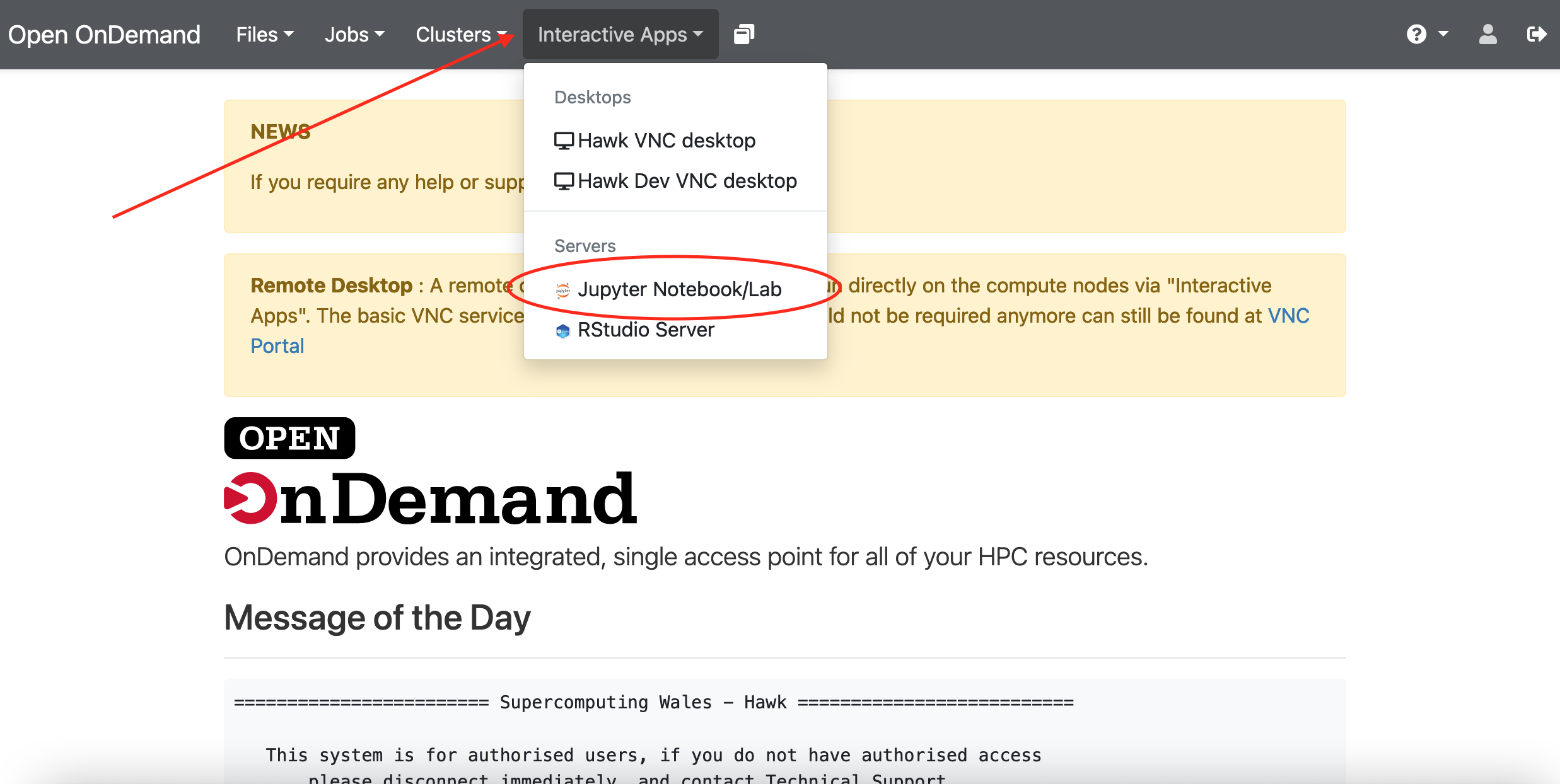
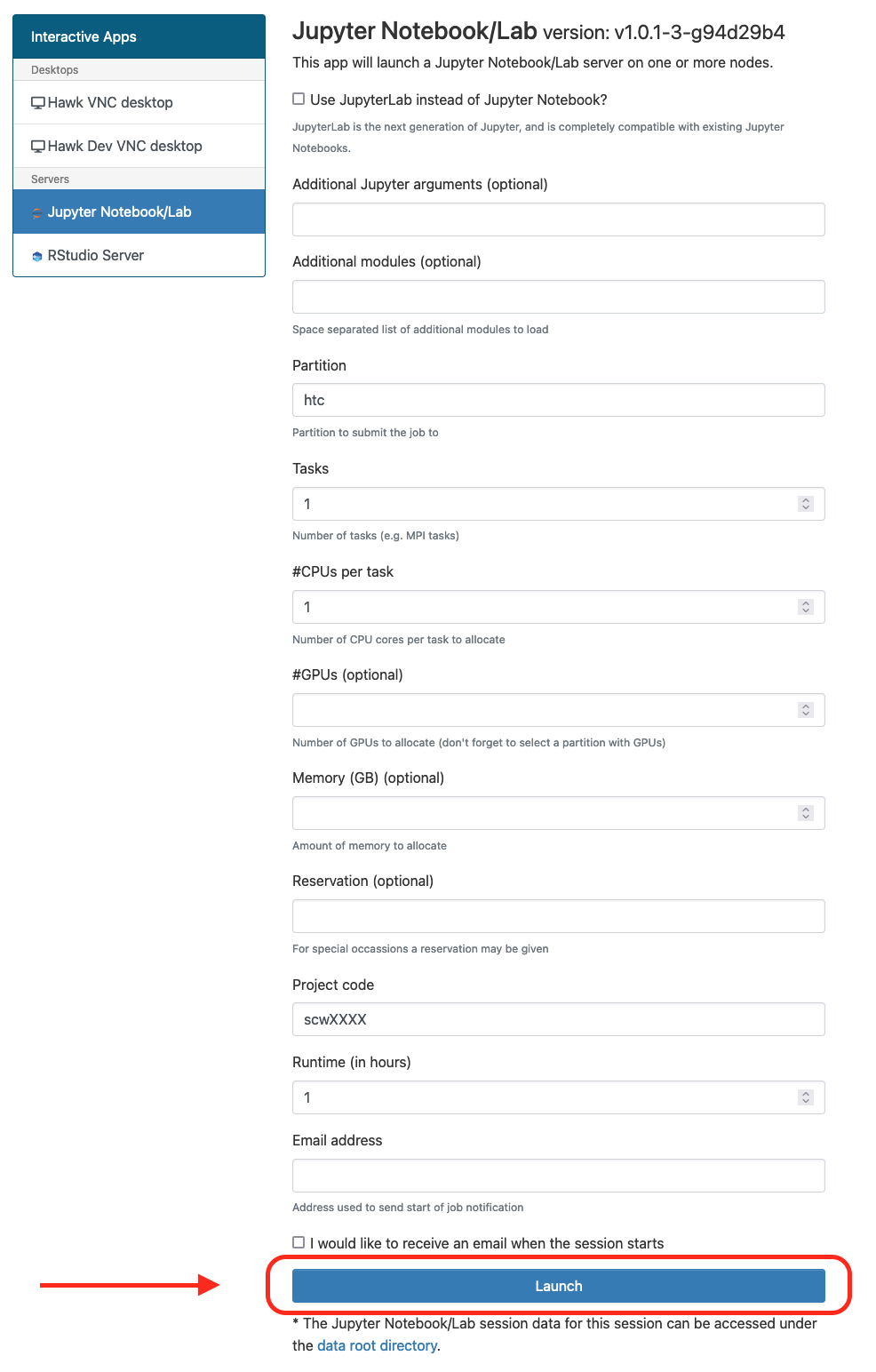
-
After submission you request will be placed on the queue and will wait for resources, hopefully for a short period, but this depends on the number of cores as well as time requested, so please be patient. At this point you can close the OnDemand website and come back at a later point to check progress or wait for the email notification if the option was selected.
Once your request is granted you should be able to see a Running message, the amount of resources granted and the time remaining.
Click Connect to Jupyter to launch the Jupyter in a new web browser tab.
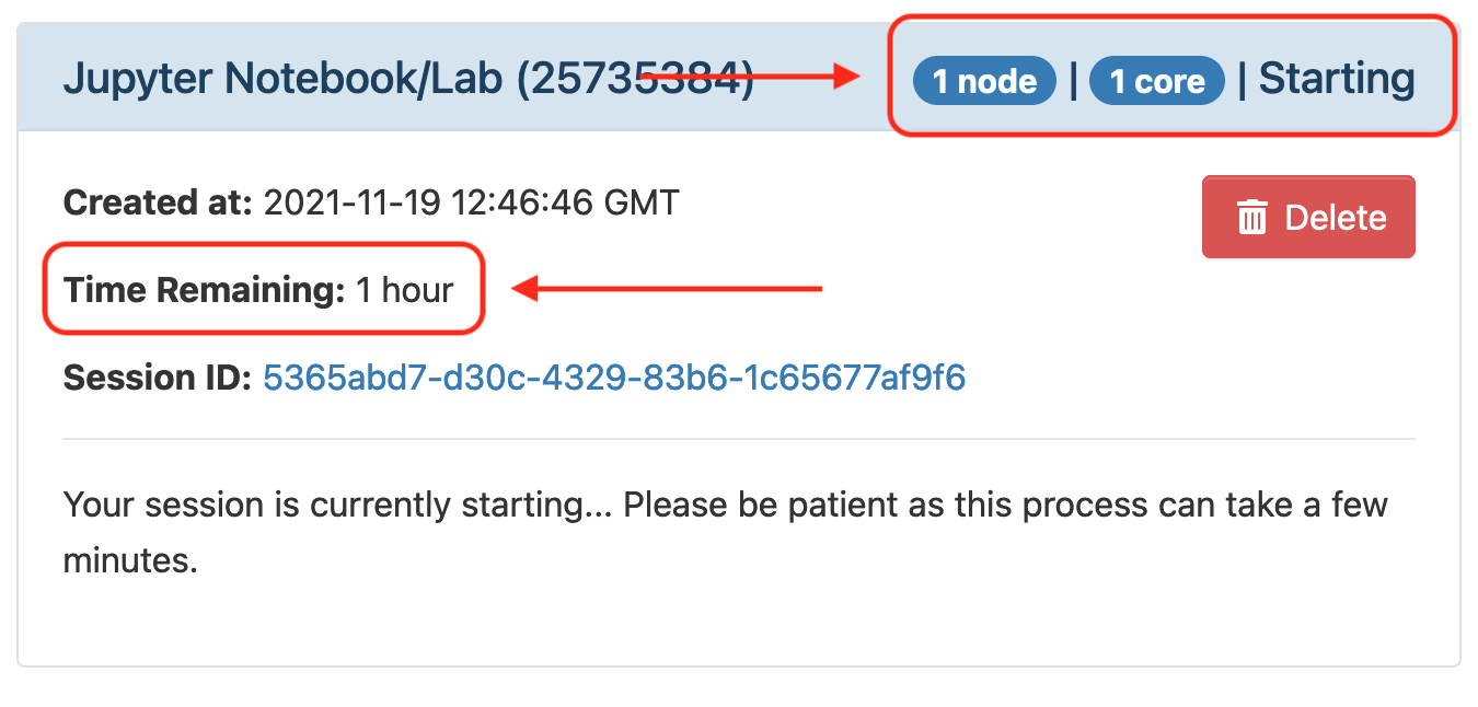
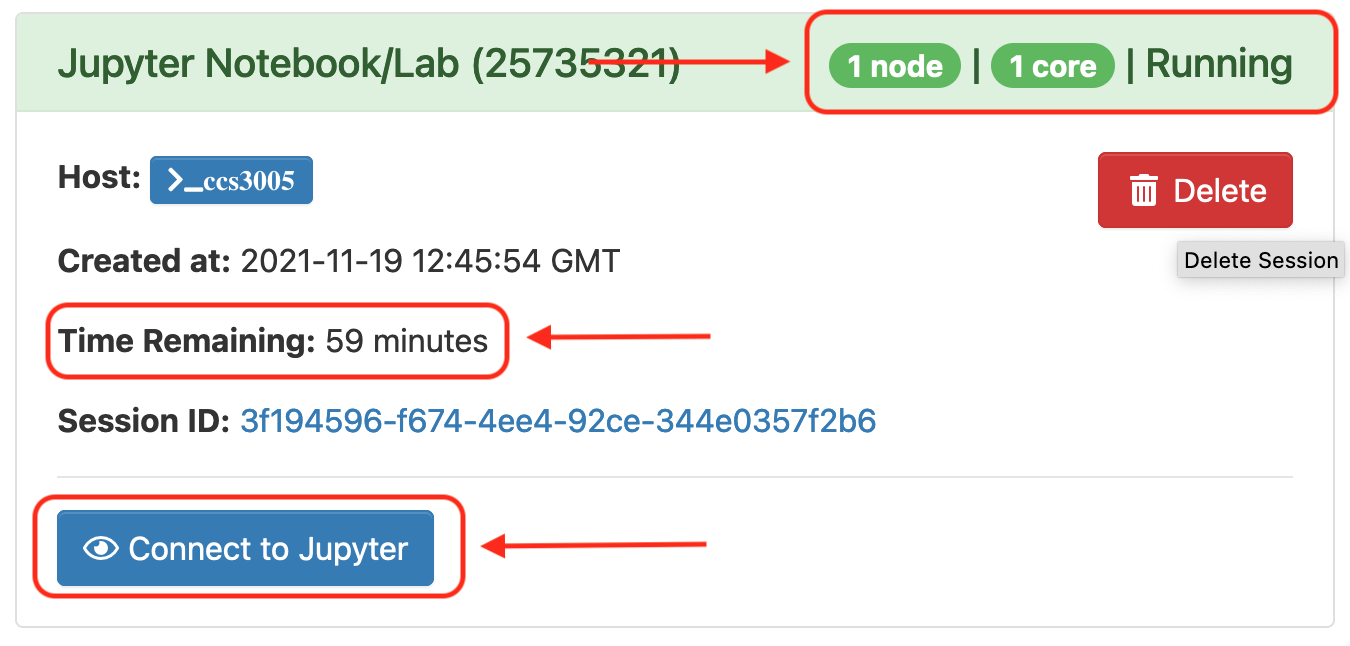
-
You should now have the familiar interface of Jupyter Notebooks in front of you. It will show the documents and directories in your user account on Hawk. To create a new Notebook, go to the dropdown menu New on the right side and click on Python 3 (ipykernel). A new tab will open with a new notebook ready for you to start working.
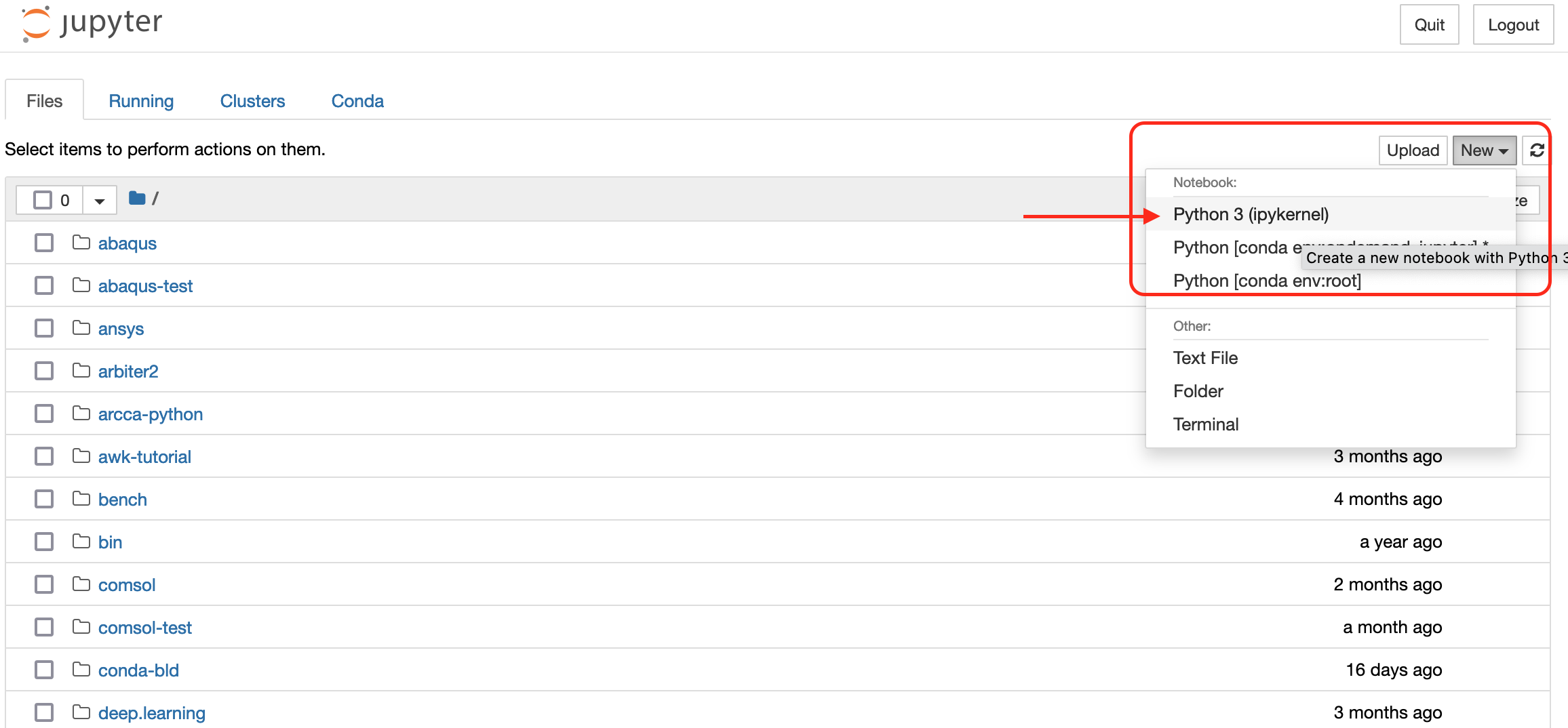
Copying data
To keep working on Hawk with the Notebooks we have written locally in our Desktop computer we need to transfer them over. Depending on our platform we can do this in a couple of ways:
On Windows you can use MobaXterm to transfer files to Hawk from your local computer.
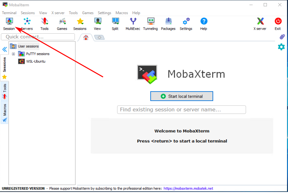 Click on Session to open the different connection methods available in MobaXterm |
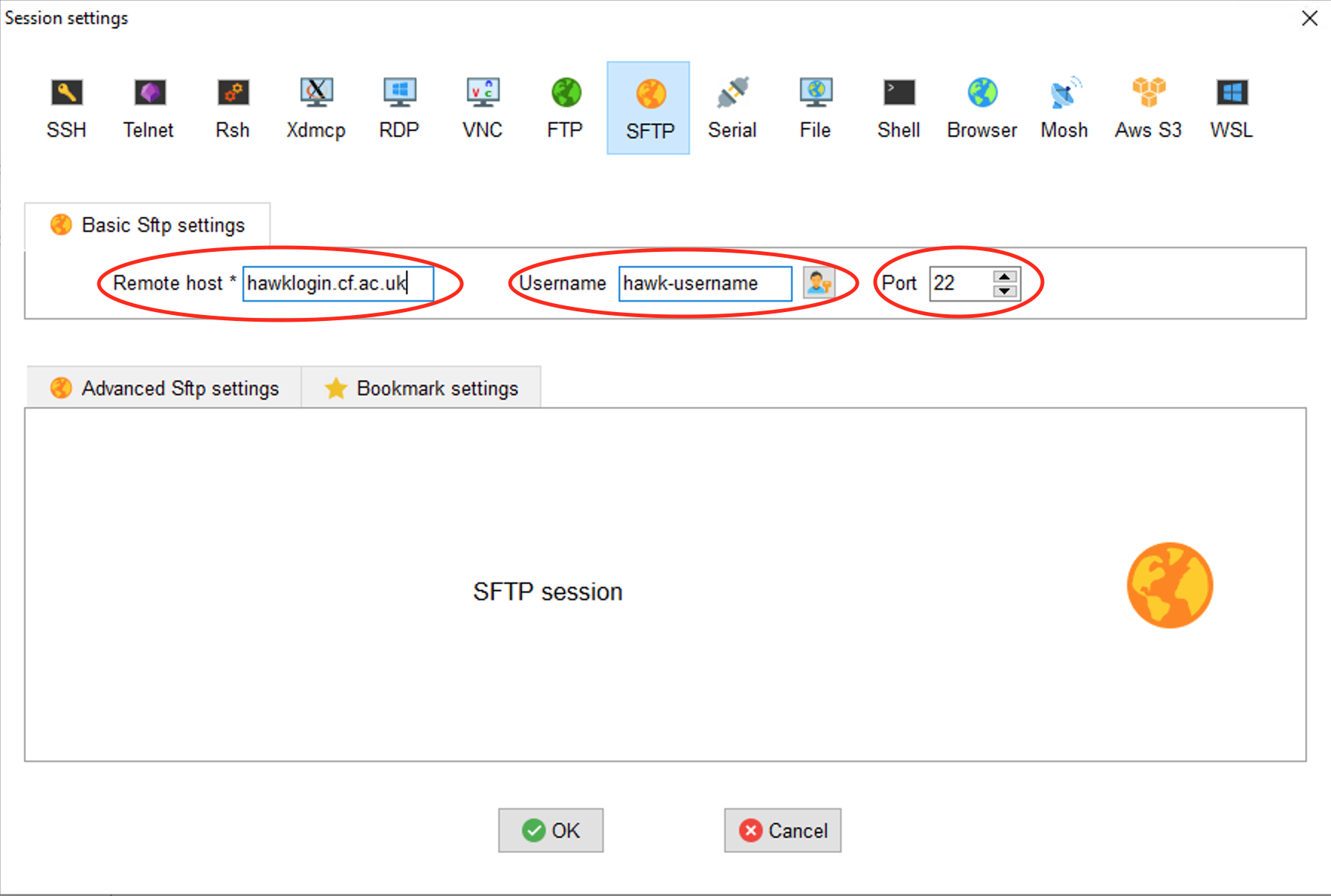 Select SFTP and enter the Remote Host (hawklogin.cf.ac.uk) and your Hawk username |
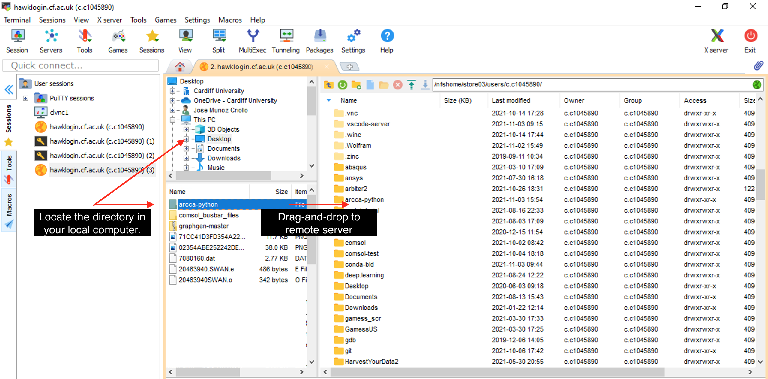 Locate the directory in your local computer and drag and drop to the remote server on the right pane. |
MacOS and Linux provide the command scp -r that can be used to recursively copy your work directory over to your home directory in Hawk:
  $ scp -r arcca-python hawk-username@hawklogin.cf.ac.uk:/home/hawk-username
  python-novice-inflammation-code.zip           100% 7216   193.0KB/s   00:00
  Untitled.ipynb                                100%   67KB 880.2KB/s   00:00
  inflammation.png                              100%   13KB 315.6KB/s   00:00
  argv_list.py                                  100%   42     0.4KB/s   00:00
  readings_08.py                                100% 1097    10.6KB/s   00:00
  readings_09.py                                100%  851    24.8KB/s   00:00
With OnDemand you can also download and upload files to Hawk. In this
example we will upload the directory with the Jupyter Notebooks we have
created so far. Go to Files and select the directory where you wish to
upload the files (our home directory in this case), then select Upload
and locate the directory in your local computer. Once uploaded, the files
should be available on Hawk:
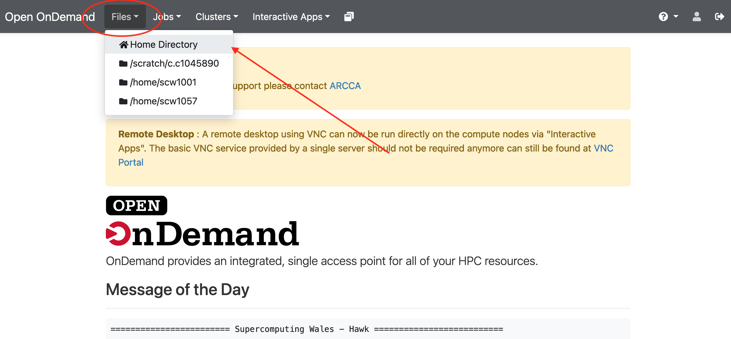 |
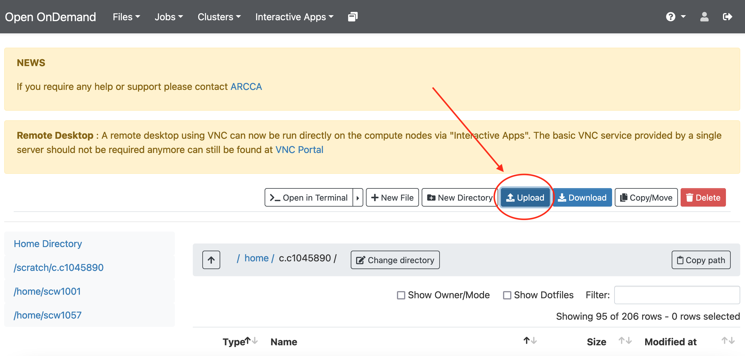 |
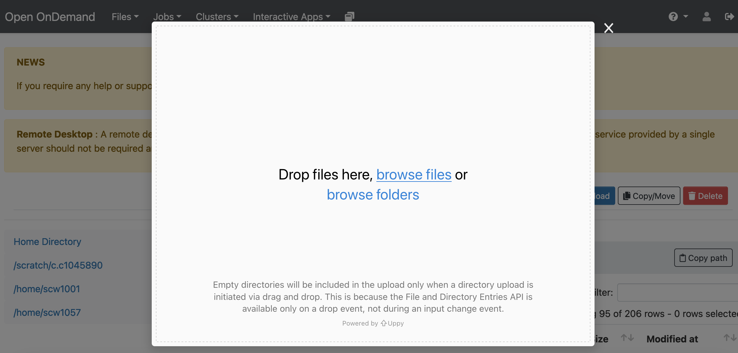 |
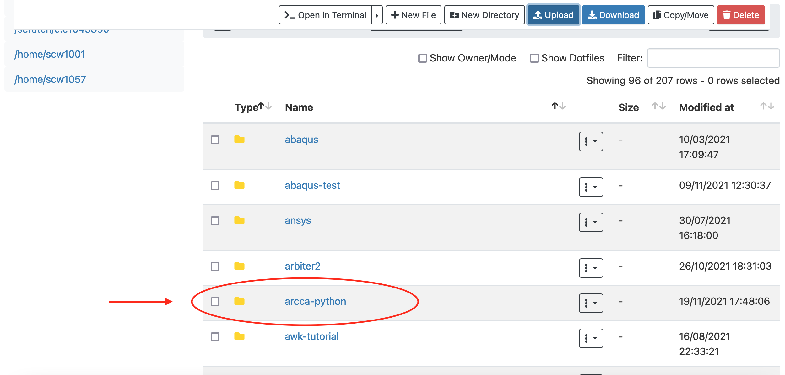 |
Setup your Jupyter Notebook work environment
Depending on how you started your Jupyter Notebook you should have access to
some default packages. But these are not guaranteed to be the same (this also
applies for the version of Python) between the OnDemand and the ssh tunnel
methods. Moreover, it is unlikely that the remote HPC system would provide
every package you need by default.
Installing Python libraries
The recommended approach is to create a conda virtual environment with a
environemnt.yml file which includes a list of all packages (and versions)
needed for your work. This file can be created and used in your local computer
and then copied to Hawk to reproduce the same environment. An example file is:
name: my-conda-env
dependencies:
  - python=3.9.2
  - numpy
  - pandas
  - ipykernel
The package ipykernel is required here to make the environment reachable from
Jupyter Notebooks. You can find more about creating an environment.yml file
in the Anaconda documentation.
On Hawk you need to first load Anaconda:
$ module load anaconda/2020.02
$ source activate
$ which conda
/apps/languages/anaconda/2020.02/bin/conda
And then proceed to install the virtual environment:
$ conda env create -f environment.yml
...
libffi-3.3           | 50 KB     | ##################################### | 100%
numpy-1.21.2         | 23 KB     | ##################################### | 100%
pandas-1.3.4         | 9.6 MB    | ##################################### | 100%
mkl-2021.4.0         | 142.6 MB  | ##################################### | 100%
six-1.16.0           | 18 KB     | ##################################### | 100%
Preparing transaction: done
Verifying transaction: done
Executing transaction: done
#
# To activate this environment, use
#
#     $ conda activate my-conda-env
#
# To deactivate an active environment, use
#
#     $ conda deactivate
We can then follow the instructions printed at the end of the installation process to activate our environment:
$ conda activate my-conda-env
$ which python
~/.conda/envs/my-conda-env/bin/python
We can further confirm the version of Python used by the environment:
$ python --version
Python 3.9.2
To deactivate the environment and return to the default Python provided by the system (or the loaded module):
$ conda deactivate
$ python --version
Python 3.7.6
Using an Anaconda virtual environment from Jupyter Notebooks
We can access our newly installed Anaconda environment from Jupyter Notebooks
on OnDemand. For this, create a new session and when the resources are granted
click on Connect to Jupyter. On Jupyter Lab you might be asked to choose
which kernel to start, if so, select the name given to your virtual environment
(my-conda-env) in this example:
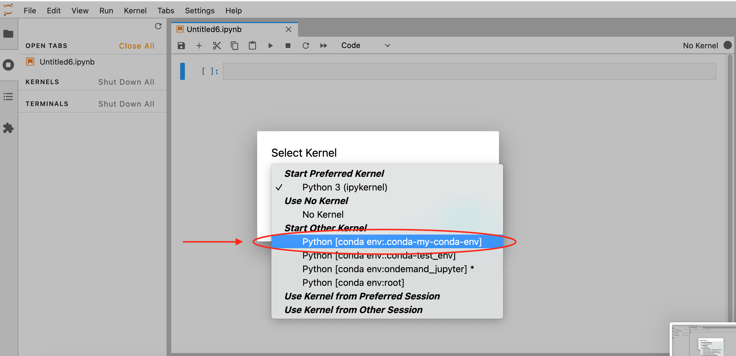
If another kernel is loaded by default, you can still change it by clicking on the top right corner of your Notebook, a similar menu should appear:
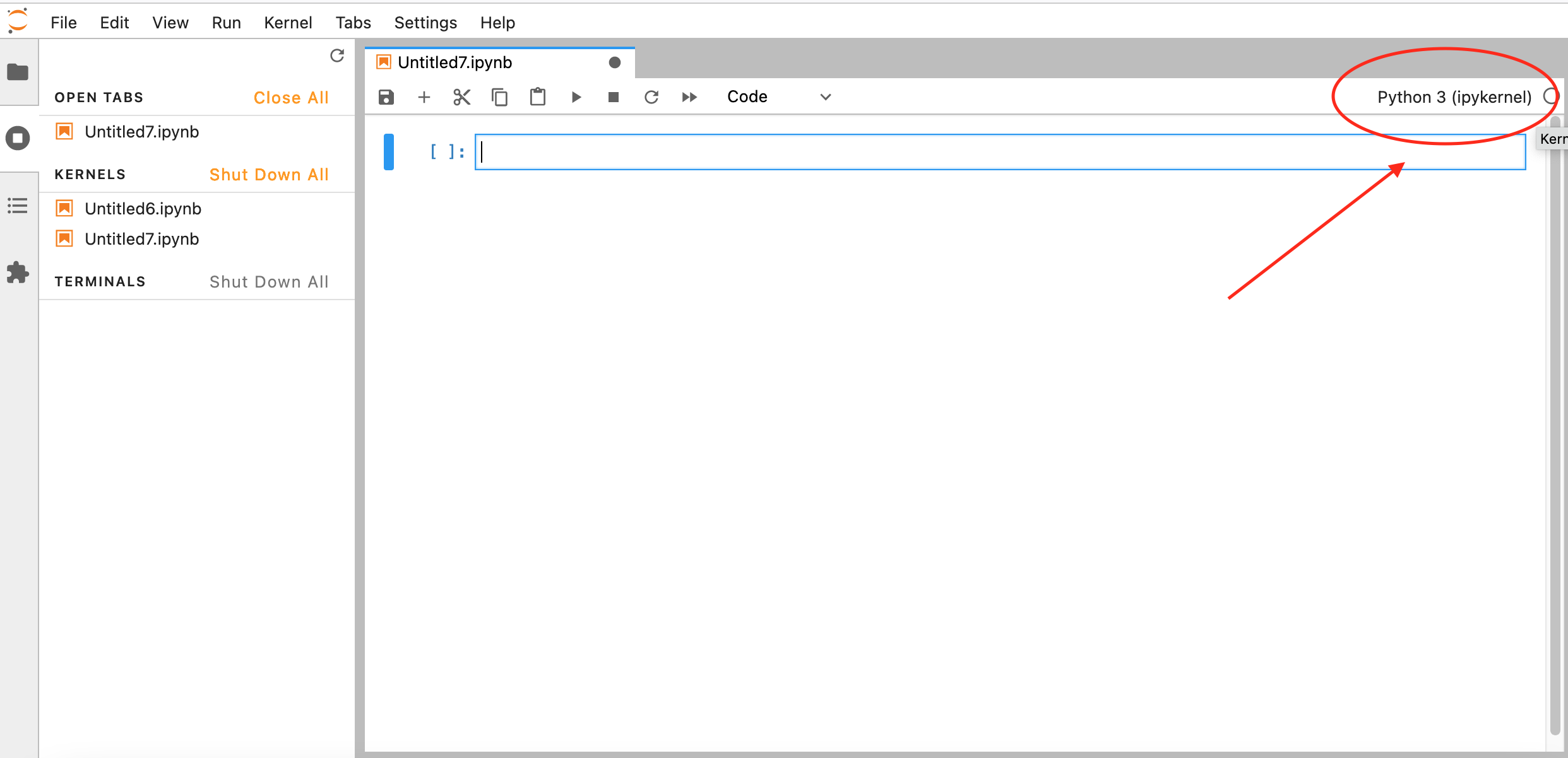 |
|
If all goes well you should be able to confirm the Python versions and path, as well as the location of the installed libraries:
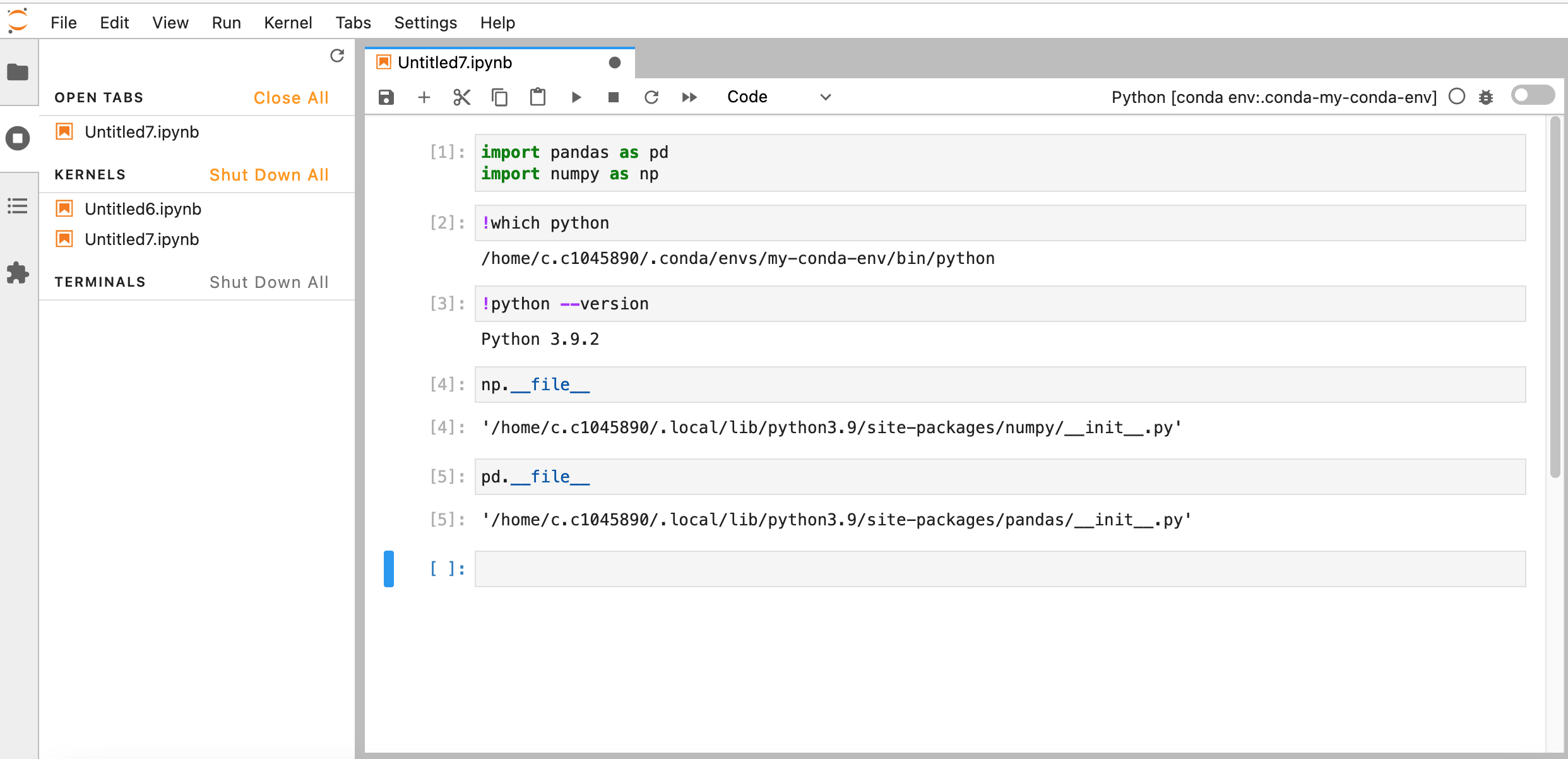
At this point you should have all the packages required to continue working on Hawk as if you were working on your local computer.
A more efficient approach
During these examples we have been requesting only 1 CPU when we launch our Jupyter Notebook and that, hopefully, has caused our request to be fulfilled fairly quickly. However, there will be a point where 1 CPU is no longer enough (maybe the application has become more complex or there is more data to analyse, and memory requirements have increased). At that point you can modify the requirements and increase the number of CPUS, memory, time or devices (GPUs). One point to keep in mind when increasing requirements is that this will impact the time it takes for the system scheduler to deliver your request and allocate you the resources, the higher the requirements, the longer it will take.
When the time spent waiting in queue becomes excessive it is worth considering moving away from the Jupyter Notebook workflow towards a more traditional Python script approach (recommended for HPC systems). The main difference between them is that while Jupyter Notebooks is ideal for the development stages of a project (since you can test things out in real time and debug if needed), the Python script approach is better suited for the production stages where the needed for supervision and debugging is reduced. Python scripts also have the advantage, on HPC systems, of being able to be queued for resources and automatically executed when these are granted without you needing to be logged in the system.
So, how do we actually transfer our Jupyter Notebook to a Python script? Fortunately, Jupyter Notebook developers thought of this requirement and added a convenient export method to the Notebooks (the menus might be different depending on if Jupyter Notebooks or Jupyter Lab was launched from OnDemand):
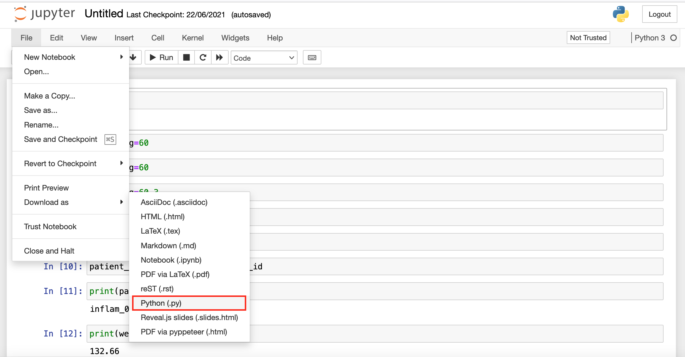 |
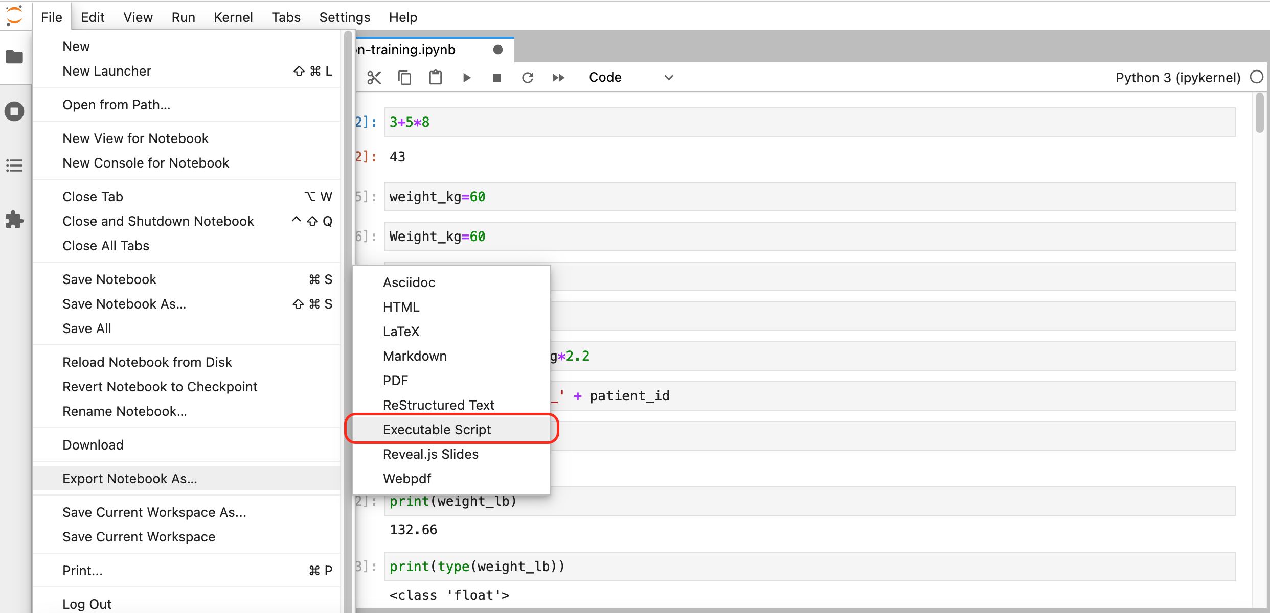 |
| Download from Jupyter Notebook | Download from Jupyter Lab |
After choosing an appropriate name and saving the file, we should have a Python script (a text file) with entries similar to:
#!/usr/bin/env python
# coding: utf-8

# In[1]:


3 + 5 * 8


# In[2]:


weight_kg=60
Notice the # In[X]: that mark the position of corresponding cells in our
Jupyter Notebook and are kept for reference. We can keep them in place, they
won’t cause any trouble as they are included as comments (due to the initial
#), but if we wanted to remove them we could do it by hand or more
efficiently by using the command line tool sed to find and delete lines that
start with the characters # [ and to delete empty lines (^ is used by sed
to indicate the beginning of a line and $ to indicate the end):
(from this point onwards we move away from Jupyter Notebooks and start typing commands on a terminal connected to Hawk)
sed -e '/# In/d' -e '/^$/d' lesson1.py > lesson1_cleaned.py
This will produce the lesson1_cleaned.py file with entries similar to:
#!/usr/bin/env python
# coding: utf-8
3+5+8
weight_kg=60
Now that we have our Python script, we need to create an additional file (job script) to place it in the queue (submit the job). Make sure to remove any commands from the Python script that might need additional confirmation or user interaction as you won’t be able to provide it with this method of execution. The following is the content a job script that is equivalent to how we have been requesting resources through OnDemand:
#!/bin/bash

#SBATCH -J test             # job name
#SBATCH -n 1                # number of tasks needed
#SBATCH -p htc              # partition
#SBATCH --time=01:00:00     # time limit
#SBATCH -A scwXXXX          # account number

set -eu

module purge
module load anaconda/2020.02
module list

# Load conda
source activate

# Load our environment
conda activate my-conda-env

which python
python --version

python my-python-script.py
To submit (put it queue) the above script, on Hawk:
$ sbatch my-job-script.sh
Submitted batch job 25859860
You can query the current state of this job with:
$ squeue -u $USER
    JOBID       PARTITION    NAME    USER      ST    TIME  NODES NODELIST(REASON)
    25860025    htc          test    c.xxxxxxx PD    0:00      1 ccs3004
This particular job might not spend a long time in queue and the above output
might not show it, but on completion there should be a slurm-<job-id>.out
created in the current directory with the output produced by our script.
There is a lot more to know about working with HTC systems and job schedulers, once you are ready to go this route, take a look at our documentation and training courses on these topics:
- Supercomputing for Beginners: Why use HPC? Accessing systems, using SLURM, loading software, file transfer and optimising resources.
- Slurm: Advanced Topics: Additional material to interface with HPC more effectively.
Need help?
If during the above steps you found any issues or have doubts regarding your specific work environment, get in touch with us at arcca-help@cardiff.ac.uk.
Key Points
It is possible to use Jupyter Notebooks on Hawk via OnDemand and ssh tunnels.
The recommended method to setup your work environment (installing libraries) is using Anaconda virtual environments.
Include the library ipykernel to make the environment reachable from Jupyter Notebooks
Use Jupyter Notebooks in the early (development) stages of your project when lots of debugging are necessary. Move towards automated Python scripts in later stages and submit them via SLURM job scripts.